
Note
Go to the end to download the full example code.
Auditing identifiability before reading learned physics fields#
This application treats the bounds-versus-ridge analysis as a scientific audit, not as a side figure.
The central question is practical:
When GeoPrior learns effective fields such as \(K\), \(S_s\), \(H_d\), and :math:` au`, which parts of that field story are safe to interpret, and which parts require caution?
The page therefore does three things.
It explains why the closure itself creates a ridge-like non-identifiability pathway.
It rebuilds the reported synthetic audit snapshot from a compact reference table.
It ends with an interpretation protocol that tells the reader what is safe to claim from the fitted fields.
Why this matters#
A forecasting model can be accurate and still remain partly non-identifiable in its internal decomposition. That is not a failure by itself. It becomes a problem only when users read a closure-constrained field as if it were a uniquely recovered hydrogeological truth.
This application shows how GeoPrior avoids that mistake: it pairs the forecasting workflow with explicit guardrails based on ridge diagnostics and bound saturation.
from __future__ import annotations

import numpy as np
import pandas as pd
import matplotlib.pyplot as plt
from matplotlib.colors import LinearSegmentedColormap
from matplotlib.patches import FancyBboxPatch

N_RUNS = 50
RIDGE_THR = 2.0

BOUND_HITS = pd.DataFrame(
    {
        "parameter": [
            r"$K_{\max}$",
            r"$K_{\min}$",
            r"$\tau_{\min}$",
            r"$\tau_{\max}$",
            r"$H_{d,\max}$",
            r"$H_{d,\min}$",
        ],
        "count": [1, 1, 1, 1, 17, 1],
    }
)
BOUND_HITS["fraction"] = BOUND_HITS["count"] / float(N_RUNS)

FAILURE_MATRIX = pd.DataFrame(
    {
        "No ridge": [25, 18],
        "Strong ridge": [5, 2],
    },
    index=["Not clipped", "Clipped"],
)


SAFE_READING = pd.DataFrame(
    [
        {
            "bucket": "Green — stable audit",
            "count": 25,
            "fraction": 0.50,
            "meaning": (
                "Neither clipped nor ridge-dominated. "
                "Best zone for interpretation."
            ),
        },
        {
            "bucket": "Amber — clipped only",
            "count": 18,
            "fraction": 0.36,
            "meaning": (
                "A boundary is active, so the field is still usable "
                "mainly in relative terms."
            ),
        },
        {
            "bucket": "Amber — ridge only",
            "count": 5,
            "fraction": 0.10,
            "meaning": (
                "The closure admits competing decompositions. "
                "Trust the effective timescale more than the split."
            ),
        },
        {
            "bucket": "Red — clipped and ridge",
            "count": 2,
            "fraction": 0.04,
            "meaning": (
                "This is the strongest caution case. Avoid literal "
                "component interpretation."
            ),
        },
    ]
)


def build_reference_snapshot() -> pd.Series:
    """Return the compact audit snapshot.

    The values come from the reported 50-realization SM3
    reference audit used to summarize clipping and ridge
    behaviour in a closure-constrained setting.
    """
    strong_ridge = 7
    clipped_any = 20
    clipped_and_ridge = 2
    hdmax = 17

    return pd.Series(
        {
            "n_runs": N_RUNS,
            "strong_ridge_count": strong_ridge,
            "strong_ridge_frac": strong_ridge / float(N_RUNS),
            "clipped_any_count": clipped_any,
            "clipped_any_frac": clipped_any / float(N_RUNS),
            "clipped_and_ridge_count": clipped_and_ridge,
            "clipped_and_ridge_frac": (
                clipped_and_ridge / float(N_RUNS)
            ),
            "hdmax_count": hdmax,
            "hdmax_frac": hdmax / float(N_RUNS),
        }
    )


def make_ridge_demo(
    n_stable: int = 55,
    n_ridge: int = 20,
    n_outliers: int = 10,
    seed: int = 7,
) -> pd.DataFrame:
    """Create a synthetic ridge-geometry teaching dataset.

    This is not intended to reproduce the original SM3 rows.
    It is only a geometric teaching aid for the closure ridge
    relation

    .. math::

       \delta_K \approx \delta_{S_s} + 2\,\delta_{H_d}.
    """
    rng = np.random.default_rng(seed)

    x_stable = rng.normal(0.0, 0.45, size=n_stable)
    y_stable = x_stable + rng.normal(0.0, 0.12, size=n_stable)
    tag_stable = ["near ridge"] * n_stable

    x_ridge = rng.normal(0.8, 0.65, size=n_ridge)
    y_ridge = x_ridge + rng.normal(0.0, 0.28, size=n_ridge)
    tag_ridge = ["ridge drift"] * n_ridge

    x_out = rng.uniform(-1.6, 2.6, size=n_outliers)
    y_out = rng.uniform(-1.8, 2.8, size=n_outliers)
    tag_out = ["off-ridge"] * n_outliers

    x = np.r_[x_stable, x_ridge, x_out]
    y = np.r_[y_stable, y_ridge, y_out]
    tag = tag_stable + tag_ridge + tag_out

    df = pd.DataFrame(
        {
            "ridge_x": x,
            "ridge_y": y,
            "tag": tag,
        }
    )
    df["ridge_abs"] = np.abs(
        df["ridge_y"] - df["ridge_x"]
    )
    return df


def build_interpretation_cards() -> list[dict[str, str]]:
    """Return short interpretation cards for plotting."""
    return [
        {
            "title": "Safe claim",
            "body": (
                "The effective timescale and the overall reduced-"
                "physics behaviour remain interpretable when the "
                "audit is green."
            ),
        },
        {
            "title": "Caution claim",
            "body": (
                "When only one warning appears, interpret maps in "
                "relative or regional terms rather than as exact "
                "component recovery."
            ),
        },
        {
            "title": "Unsafe claim",
            "body": (
                "If clipping and strong ridge co-occur, avoid a "
                "literal reading of K, Ss, Hd, or tau as uniquely "
                "identified local truth."
            ),
        },
    ]


snapshot = build_reference_snapshot()
ridge_demo = make_ridge_demo()
Problem framing#
The reduced closure used by GeoPrior links the learned timescale to effective conductivity, storage, and drainage thickness:
In log-offset form, this means that a positive shift in \(K\) can be compensated by a coordinated shift in \(S_s\) and \(H_d\). That compensation pathway is the ridge. The model can therefore remain dynamically consistent while still allowing multiple internal decompositions.
This is why the application starts with interpretation guardrails rather than with a forecast score.
print("Reference audit snapshot:\n")
print(snapshot.round(3).to_string())

print("\nFailure-mode buckets:\n")
print(
    SAFE_READING[["bucket", "count", "fraction"]]
    .assign(fraction=lambda d: 100.0 * d["fraction"])
    .rename(columns={"fraction": "fraction_pct"})
    .round(1)
    .to_string(index=False)
)
Reference audit snapshot:

n_runs                     50.00
strong_ridge_count          7.00
strong_ridge_frac           0.14
clipped_any_count          20.00
clipped_any_frac            0.40
clipped_and_ridge_count     2.00
clipped_and_ridge_frac      0.04
hdmax_count                17.00
hdmax_frac                  0.34

Failure-mode buckets:

                 bucket  count  fraction_pct
   Green — stable audit     25          50.0
   Amber — clipped only     18          36.0
     Amber — ridge only      5          10.0
Red — clipped and ridge      2           4.0
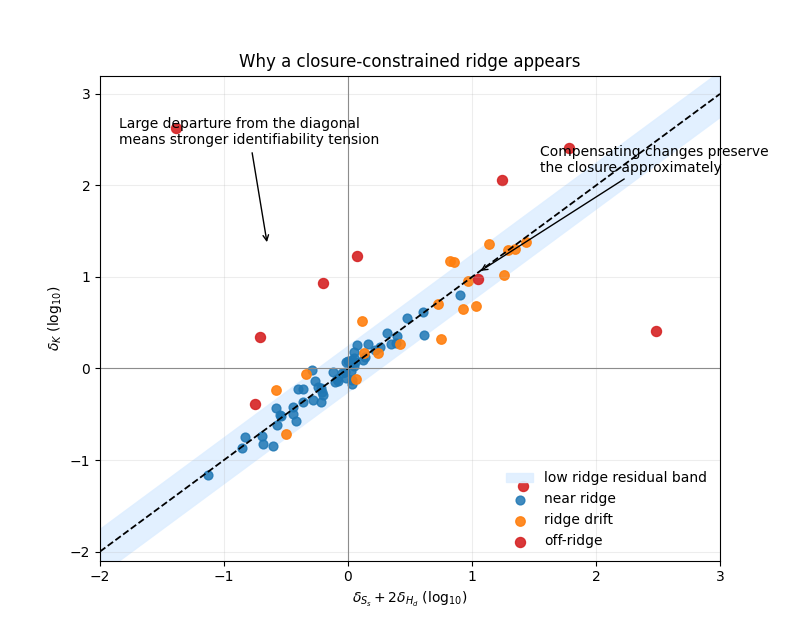
Geometric view of the ridge#
The first plot is intentionally conceptual. It teaches the geometry of the diagnostic before the page moves to the reported audit counts.
The horizontal axis is \(\delta_{S_s} + 2\delta_{H_d}\) and the vertical axis is \(\delta_K\). Points close to the 1:1 diagonal have a small ridge residual, meaning the closure can move along the diagonal while preserving nearly the same effective timescale.
In practice, this means the model may estimate an effective \(\tau\) more robustly than it estimates every component of the decomposition separately.
fig, ax = plt.subplots(figsize=(8.0, 6.3))

xmin, xmax = -2.0, 3.0
xx = np.linspace(xmin, xmax, 300)

ax.fill_between(
    xx,
    xx - 0.25,
    xx + 0.25,
    color="#dfefff",
    alpha=0.9,
    label="low ridge residual band",
)
ax.plot(xx, xx, linestyle="--", linewidth=1.3, color="black")
ax.axhline(0.0, linewidth=0.8, color="0.55")
ax.axvline(0.0, linewidth=0.8, color="0.55")

styles = {
    "near ridge": dict(color="#1f77b4", s=40, alpha=0.85),
    "ridge drift": dict(color="#ff7f0e", s=46, alpha=0.90),
    "off-ridge": dict(color="#d62728", s=52, alpha=0.92),
}

for tag, group in ridge_demo.groupby("tag", sort=False):
    ax.scatter(
        group["ridge_x"],
        group["ridge_y"],
        label=tag,
        **styles[tag],
    )

ax.annotate(
    "Compensating changes preserve\n"
    "the closure approximately",
    xy=(1.05, 1.05),
    xytext=(1.55, 2.15),
    arrowprops=dict(arrowstyle="->", linewidth=1.0),
    fontsize=10,
)

ax.annotate(
    "Large departure from the diagonal\n"
    "means stronger identifiability tension",
    xy=(-0.65, 1.35),
    xytext=(-1.85, 2.45),
    arrowprops=dict(arrowstyle="->", linewidth=1.0),
    fontsize=10,
)

ax.set_xlim(xmin, xmax)
ax.set_ylim(-2.1, 3.2)
ax.set_xlabel(r"$\delta_{S_s} + 2\delta_{H_d}$ (log$_{10}$)")
ax.set_ylabel(r"$\delta_K$ (log$_{10}$)")
ax.set_title("Why a closure-constrained ridge appears")
ax.grid(alpha=0.22)
ax.legend(frameon=False, loc="lower right")
<matplotlib.legend.Legend object at 0x749e66e8c680>
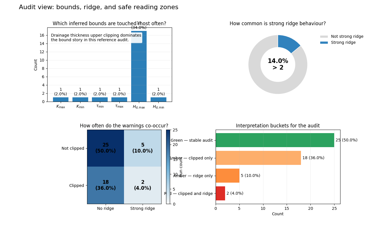
Rebuild the reference audit snapshot#
The next figure uses the reported 50-realization summary to answer a more operational question:
Which warning appears most often?
How frequent is strong ridge behaviour?
How often do clipping and strong ridge occur together?
This is the audit view a careful reader should consult before treating the learned fields as literal hydrogeologic estimates.
fig = plt.figure(figsize=(13.2, 8.0))
grid = fig.add_gridspec(2, 2, wspace=0.35, hspace=0.38)

ax_a = fig.add_subplot(grid[0, 0])
ax_b = fig.add_subplot(grid[0, 1])
ax_c = fig.add_subplot(grid[1, 0])
ax_d = fig.add_subplot(grid[1, 1])

# (a) bound hits
xb = np.arange(len(BOUND_HITS))
bars = ax_a.bar(
    xb,
    BOUND_HITS["count"],
    color="#2c7fb8",
)
ax_a.set_xticks(xb, BOUND_HITS["parameter"])
ax_a.set_ylabel("Count")
ax_a.set_title("Which inferred bounds are touched most often?")
ax_a.grid(axis="y", alpha=0.22)

for bar, frac in zip(
    bars,
    BOUND_HITS["fraction"],
    strict=False,
):
    h = bar.get_height()
    ax_a.text(
        bar.get_x() + bar.get_width() / 2.0,
        h + 0.3,
        f"{int(h)}\n({100.0 * frac:.1f}%)",
        ha="center",
        va="bottom",
        fontsize=10,
    )

ax_a.text(
    0.03,
    0.92,
    "Drainage thickness upper clipping dominates\n"
    "the bound story in this reference audit.",
    transform=ax_a.transAxes,
    va="top",
    fontsize=10,
    bbox=dict(
        boxstyle="round,pad=0.25",
        facecolor="white",
        alpha=0.9,
        linewidth=0.0,
    ),
)

# (b) strong ridge prevalence
strong = int(snapshot["strong_ridge_count"])
not_strong = N_RUNS - strong
vals = [not_strong, strong]
labels = ["Not strong ridge", "Strong ridge"]
colors = ["#d9d9d9", "#3182bd"]

wedges, _ = ax_b.pie(
    vals,
    startangle=90,
    colors=colors,
    wedgeprops=dict(width=0.42, edgecolor="white"),
)
ax_b.set_title("How common is strong ridge behaviour?")
ax_b.text(
    0.0,
    0.0,
    f"{100.0 * strong / N_RUNS:.1f}%\n> {RIDGE_THR:g}",
    ha="center",
    va="center",
    fontsize=15,
    fontweight="bold",
)
ax_b.legend(
    wedges,
    labels,
    frameon=False,
    bbox_to_anchor=(1.02, 0.95),
    loc="upper left",
)

# (c) clipping vs ridge matrix
mat = FAILURE_MATRIX.to_numpy()
cm = LinearSegmentedColormap.from_list(
    "audit_matrix",
    ["#f7f7f7", "#6baed6", "#08306b"],
)
im = ax_c.imshow(mat, cmap=cm, vmin=0, vmax=25)
ax_c.set_xticks([0, 1], FAILURE_MATRIX.columns)
ax_c.set_yticks([0, 1], FAILURE_MATRIX.index)
ax_c.set_title("How often do the warnings co-occur?")

for (i, j), val in np.ndenumerate(mat):
    ax_c.text(
        j,
        i,
        f"{val}\n({100.0 * val / N_RUNS:.1f}%)",
        ha="center",
        va="center",
        color="black",
        fontsize=12,
        fontweight="bold",
    )

cb = fig.colorbar(im, ax=ax_c, fraction=0.046, pad=0.04)
cb.set_label("Run count")

# (d) interpretation buckets
bucket_colors = ["#2ca25f", "#fdae6b", "#fd8d3c", "#de2d26"]
ypos = np.arange(len(SAFE_READING))[::-1]
ax_d.barh(
    ypos,
    SAFE_READING["count"],
    color=bucket_colors,
)
ax_d.set_yticks(ypos, SAFE_READING["bucket"])
ax_d.set_xlabel("Count")
ax_d.set_title("Interpretation buckets for the audit")
ax_d.grid(axis="x", alpha=0.22)

for y, row in zip(ypos, SAFE_READING.itertuples(index=False), strict=False):
    ax_d.text(
        row.count + 0.3,
        y,
        f"{row.count} ({100.0 * row.fraction:.1f}%)",
        va="center",
        fontsize=10,
    )

fig.suptitle(
    "Audit view: bounds, ridge, and safe reading zones",
    x=0.05,
    ha="left",
    fontsize=16,
)
Text(0.05, 0.98, 'Audit view: bounds, ridge, and safe reading zones')
Turn diagnostics into an interpretation protocol#
A good audit should not stop at percentages. It should tell the reader what to do with those percentages.
The protocol below converts the diagnostic categories into a practical reading rule. The goal is not to decide whether the forecast is useful in a general sense, but to decide how literally the internal physics fields should be read.
Claim level |
Reading rule |
Operational meaning |
|---|---|---|
Safe claim |
The effective timescale and the overall reduced-physics behaviour remain interpretable when the audit is green. |
Discuss broad effective-field pattern and closure-consistent behaviour in a comparatively direct way. |
Caution claim |
When only one warning appears, interpret maps in relative or regional terms rather than as exact component recovery. |
Use the fields for comparison, ranking, and regional structure, but avoid literal local parameter claims. |
Unsafe claim |
If clipping and strong ridge co-occur, avoid a literal reading of \(K\), \(S_s\), \(H_d\), or \(\tau\) as uniquely identified local truth. |
Treat the decomposition as too fragile for strong local interpretation; fall back to forecast behaviour and higher-level diagnostics. |
Note
Operational takeaway: the audit does not decide whether the forecast is useful. It decides how literally the internal physics fields should be read.
plt.show()
Practical interpretation#
Four conclusions matter most.
First, the audit does not say that the model is invalid. It says that the effective timescale is the safer object to interpret, whereas the component split into K, Ss, and Hd can remain partly non-unique.
Second, the dominant warning in the reference audit is not a widespread collapse of the closure. It is upper clipping in drainage thickness. That is a much narrower message than “the physics fields are untrustworthy”.
Third, the joint red zone is small. Only a minority of runs show clipping and strong ridge together, which is exactly why the diagnostics work as guardrails rather than as a blanket rejection.
Fourth, the page clarifies the difference between forecast-level trust and component-level trust. A model can keep coherent reduced-physics dynamics and still require caution when one asks for a unique local breakdown of the closure ingredients.
From audit lesson to full reproducibility#
In a real project, the complete workflow should pair the compact bounds-versus-ridge summary with the companion SM3 identifiability plot.
geoprior plot sm3-identifiability \
  --csv results/sm3_synth_1d/sm3_synth_runs.csv \
  --metric ridge_resid \
  --k-from-tau auto
geoprior plot sm3-bounds-ridge-summary \
  --csv results/sm3_synth_1d/sm3_synth_runs.csv \
  --use any \
  --ridge-thr 2.0 \
  --paper-format
import pandas as pd
from geoprior.scripts.plot_sm3_bounds_ridge_summary import (
    compute_flags,
    infer_bounds,
    plot_sm3_bounds_ridge_summary,
)

df = pd.read_csv("results/sm3_synth_1d/sm3_synth_runs.csv")
bounds = infer_bounds(df)
flags = compute_flags(
    df,
    bounds,
    rtol=1e-6,
    ridge_thr=2.0,
)

plot_sm3_bounds_ridge_summary(
    df,
    flags=flags,
    bounds=bounds,
    ridge_thr=2.0,
    use="any",
    out="sm3-bounds-ridge-audit",
    out_json="sm3-bounds-ridge-audit.json",
    out_csv="sm3-bounds-ridge-categories.csv",
    dpi=300,
    font=10,
    show_legend=True,
    show_labels=True,
    show_ticklabels=True,
    show_title=True,
    show_panel_titles=True,
    show_panel_labels=True,
    paper_format=True,
    title=None,
)
The resulting JSON and CSV exports are important. They turn the audit into a traceable artifact that can be reviewed, compared across identifiability regimes, or attached to a model card for deployment.
Total running time of the script: (0 minutes 0.686 seconds)