Cumulative subsidence on a satellite-style map

This example teaches you how to read the GeoPrior cumulative subsidence map figure.

Many forecasting figures show either one year or one city at a time. This figure is more ambitious. It tries to answer a timeline question:

How does cumulative subsidence evolve from the validation year into the forecast years, and does that evolution look similar in both cities?

That is why this figure is useful. It combines:

• observed cumulative subsidence,

• predicted cumulative subsidence for the same year,

• future cumulative forecast maps,

• and an optional hotspot overlay.

What the figure shows

The real plotting backend builds a layout with two rows and multiple columns.

Rows

• Nansha

• Zhongshan

Columns

• observed cumulative map in year_val

• predicted cumulative map in year_val

• forecast cumulative maps in the requested future years

So the eye reads from left to right:

observed -> predicted -> future

Why cumulative maps matter

Incremental yearly maps can be useful, but cumulative maps answer a different decision-facing question:

Where has deformation accumulated the most since a baseline year?

That is often easier to communicate for risk planning, because it summarizes total burden rather than only year-to-year change.

The real script supports two input conventions:

• already cumulative values, which are rebased at the first year at or after start_year,

• or yearly increments/rates, which are accumulated.

It also auto-detects whether coordinates look like longitude / latitude or projected UTM coordinates, then converts them to web mercator for basemap display.

import tempfile
from pathlib import Path

import contextily as cx
import matplotlib.image as mpimg
import matplotlib.pyplot as plt
import numpy as np
import pandas as pd

from geoprior.scripts.plot_geocum import (
    plot_geo_cumulative_main,
)

Step 1 - Understand the figure we want to teach

The real plotting script builds a two-row comparison:

• top row: Nansha

• bottom row: Zhongshan

Inside each row, the columns read from left to right:

• validation-year observed cumulative map,

• validation-year predicted cumulative map,

• future cumulative forecast maps.

A good lesson therefore needs inputs that are visually rich enough to make those column-to-column comparisons obvious.

That is why we do not use a tiny rectangular grid here. Instead, we build denser synthetic point clouds with a more city-like footprint.

Step 2 - Build a city-shaped spatial support

A spatial lesson becomes easier to read when the point cloud already looks like an urban footprint rather than a plain box.

We do that in two stages:

1. create a dense lon/lat mesh,

2. keep only the points that fall inside a synthetic mask.

The masks below are not real administrative boundaries. They are only teaching devices that make the gallery figure look closer to a real city-scale map.

def _city_mask(
    xn: np.ndarray,
    yn: np.ndarray,
    *,
    city: str,
) -> np.ndarray:
    e1 = ((xn - 0.50) / 0.44) ** 2 + ((yn - 0.50) / 0.34) ** 2 <= 1.0
    e2 = ((xn - 0.68) / 0.24) ** 2 + ((yn - 0.56) / 0.18) ** 2 <= 1.0
    cut = ((xn - 0.18) / 0.12) ** 2 + ((yn - 0.74) / 0.14) ** 2 <= 1.0

    if city.lower().startswith("nan"):
        band = (yn > 0.22) & (yn < 0.84) & (xn > 0.08)
        return (e1 | e2 | band) & (~cut)

    e3 = ((xn - 0.36) / 0.18) ** 2 + ((yn - 0.30) / 0.14) ** 2 <= 1.0
    corridor = (
        (xn > 0.22)
        & (xn < 0.86)
        & (yn > 0.18)
        & (yn < 0.74)
    )
    return (e1 | e3 | corridor) & (~cut)

Step 3 - Build a cumulative deformation pattern

A cumulative subsidence lesson should not look flat. We therefore combine several ingredients:

• one main lobe,

• one secondary lobe,

• a weak ridge,

• a directional drift,

• and a small oscillatory term.

This gives a surface that is easy to compare across years and across cities.

def _multi_lobe_surface(
    xn: np.ndarray,
    yn: np.ndarray,
    *,
    amp: float,
    drift_x: float,
    drift_y: float,
    phase: float,
) -> np.ndarray:
    g1 = np.exp(
        -(((xn - 0.66) ** 2) / 0.018 + ((yn - 0.44) ** 2) / 0.030)
    )
    g2 = np.exp(
        -(((xn - 0.38) ** 2) / 0.040 + ((yn - 0.64) ** 2) / 0.020)
    )
    ridge = np.exp(-((yn - (0.32 + 0.22 * xn)) ** 2) / 0.018)
    wave = 0.25 * np.sin(2.6 * np.pi * xn + phase)
    wave = wave * np.cos(1.8 * np.pi * yn)
    trend = drift_x * xn + drift_y * yn
    return amp * (0.95 * g1 + 0.55 * g2 + 0.18 * ridge + 0.10 * wave)
    + trend

Step 4 - Generate validation and forecast tables

The real backend expects two tables per city:

• one validation CSV,

• one future CSV.

We keep that real schema here so the lesson teaches the true workflow and not a toy interface.

Validation rows contain:

• sample_idx

• coord_t

• coord_x

• coord_y

• subsidence_actual

• subsidence_q50

Future rows keep the same spatial columns but only need the forecast median subsidence_q50.

def _make_city_frames(
    city: str,
    *,
    lon0: float,
    lat0: float,
    amp: float,
    drift_x: float,
    drift_y: float,
    seed: int,
) -> tuple[pd.DataFrame, pd.DataFrame]:
    rng = np.random.default_rng(seed)

    nx = 58
    ny = 42

    xs = np.linspace(lon0 - 0.070, lon0 + 0.070, nx)
    ys = np.linspace(lat0 - 0.052, lat0 + 0.052, ny)

    X, Y = np.meshgrid(xs, ys)
    X = X + rng.normal(0.0, 0.0012, size=X.shape)
    Y = Y + rng.normal(0.0, 0.0010, size=Y.shape)

    xn = (X - X.min()) / (X.max() - X.min())
    yn = (Y - Y.min()) / (Y.max() - Y.min())

    keep = _city_mask(xn, yn, city=city)

    X = X[keep]
    Y = Y[keep]
    xn = xn[keep]
    yn = yn[keep]

    base = _multi_lobe_surface(
        xn,
        yn,
        amp=amp,
        drift_x=drift_x,
        drift_y=drift_y,
        phase=0.7 if city.lower().startswith("nan") else 1.6,
    )

    local_bias = 1.8 * np.sin(5.0 * xn)
    local_bias = local_bias + 1.1 * np.cos(4.0 * yn)
    structural = base + local_bias

    sample_idx = np.arange(X.size, dtype=int)
    years_val = [2020, 2021, 2022]
    years_future = [2023, 2024, 2025]

    val_rows: list[dict[str, float | int]] = []
    fut_rows: list[dict[str, float | int]] = []

    for yy in years_val:
        mult = {2020: 0.0, 2021: 0.40, 2022: 0.86}[yy]
        actual = mult * structural
        actual = actual + rng.normal(0.0, 0.65, size=X.size)
        pred = 0.985 * mult * structural + 0.18
        pred = pred + rng.normal(0.0, 0.48, size=X.size)

        for i in range(X.size):
            val_rows.append(
                {
                    "sample_idx": int(sample_idx[i]),
                    "coord_t": int(yy),
                    "coord_x": float(X[i]),
                    "coord_y": float(Y[i]),
                    "subsidence_actual": float(actual[i]),
                    "subsidence_q50": float(pred[i]),
                }
            )

    for yy in years_future:
        mult = {2023: 1.08, 2024: 1.33, 2025: 1.64}[yy]
        drift_term = 0.75 * (yy - 2022)
        drift_term = drift_term * (0.35 * xn + 0.18 * yn)
        pred = mult * structural + drift_term
        pred = pred + rng.normal(0.0, 0.58, size=X.size)

        for i in range(X.size):
            fut_rows.append(
                {
                    "sample_idx": int(sample_idx[i]),
                    "coord_t": int(yy),
                    "coord_x": float(X[i]),
                    "coord_y": float(Y[i]),
                    "subsidence_q50": float(pred[i]),
                }
            )

    return pd.DataFrame(val_rows), pd.DataFrame(fut_rows)


ns_val, ns_future = _make_city_frames(
    "Nansha",
    lon0=113.55,
    lat0=22.70,
    amp=38.0,
    drift_x=7.5,
    drift_y=3.2,
    seed=10,
)

zh_val, zh_future = _make_city_frames(
    "Zhongshan",
    lon0=113.38,
    lat0=22.52,
    amp=33.0,
    drift_x=4.4,
    drift_y=6.6,
    seed=22,
)

print("Validation rows")
print(f"  Nansha:    {len(ns_val)}")
print(f"  Zhongshan: {len(zh_val)}")
print("")
print("Future rows")
print(f"  Nansha:    {len(ns_future)}")
print(f"  Zhongshan: {len(zh_future)}")

Validation rows
  Nansha:    4155
  Zhongshan: 3477

Future rows
  Nansha:    4155
  Zhongshan: 3477

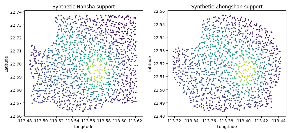
Step 5 - Preview the synthetic spatial support

Before running the final figure, it is useful to inspect the synthetic support itself.

This preview teaches an important point: dense and irregular point support usually gives a much more convincing spatial reading than a sparse classroom grid.

fig, axes = plt.subplots(figsize=(10.0, 4.6), ncols=2)

axes[0].scatter(
    ns_val.loc[ns_val["coord_t"].eq(2022), "coord_x"],
    ns_val.loc[ns_val["coord_t"].eq(2022), "coord_y"],
    c=ns_val.loc[ns_val["coord_t"].eq(2022), "subsidence_q50"],
    s=5,
)
axes[0].set_title("Synthetic Nansha support")
axes[0].set_xlabel("Longitude")
axes[0].set_ylabel("Latitude")

axes[1].scatter(
    zh_val.loc[zh_val["coord_t"].eq(2022), "coord_x"],
    zh_val.loc[zh_val["coord_t"].eq(2022), "coord_y"],
    c=zh_val.loc[zh_val["coord_t"].eq(2022), "subsidence_q50"],
    s=5,
)
axes[1].set_title("Synthetic Zhongshan support")
axes[1].set_xlabel("Longitude")
axes[1].set_ylabel("Latitude")

fig.tight_layout()

Step 5b - Build a hotspot overlay table

The backend can optionally overlay forecast hotspots.

For the lesson, we define a hotspot very simply: the highest forecast median values in a selected year.

This is a good teaching choice because it keeps the hotspot logic transparent. Readers can immediately understand that the overlay is derived from the strongest forecasted cumulative burden.

def _top_hotspots(
    city: str,
    fut_df: pd.DataFrame,
    *,
    years: list[int],
    n_top: int,
) -> pd.DataFrame:
    rows: list[pd.DataFrame] = []

    for yy in years:
        sub = fut_df.loc[fut_df["coord_t"].eq(yy)].copy()
        sub = sub.nlargest(n_top, "subsidence_q50").copy()
        sub["city"] = city
        sub["year"] = int(yy)
        sub["kind"] = "forecast"
        sub["score"] = sub["subsidence_q50"]
        rows.append(
            sub[
                [
                    "city",
                    "year",
                    "kind",
                    "coord_x",
                    "coord_y",
                    "score",
                ]
            ]
        )

    return pd.concat(rows, ignore_index=True)


hotspots = pd.concat(
    [
        _top_hotspots("Nansha", ns_future, years=[2024, 2025], n_top=18),
        _top_hotspots(
            "Zhongshan",
            zh_future,
            years=[2024, 2025],
            n_top=18,
        ),
    ],
    ignore_index=True,
)

print("\nHotspot rows")
print(hotspots.head().to_string(index=False))

Hotspot rows
  city  year     kind  coord_x  coord_y   score
Nansha  2024 forecast 113.5723  22.6956 58.2734
Nansha  2024 forecast 113.5742  22.6943 57.5127
Nansha  2024 forecast 113.5715  22.6946 57.3731
Nansha  2024 forecast 113.5691  22.6946 57.0293
Nansha  2024 forecast 113.5734  22.6939 56.9043

Step 6 - Write temporary CSV files

Sphinx Gallery examples should teach the real file contract of the plotting script.

For that reason, we write temporary CSV files and pass them to the backend exactly as a workflow would do.

tmp_dir = Path(tempfile.mkdtemp(prefix="gp_sg_geo_cum_dense_"))

ns_val_csv = tmp_dir / "nansha_val.csv"
zh_val_csv = tmp_dir / "zhongshan_val.csv"
ns_future_csv = tmp_dir / "nansha_future.csv"
zh_future_csv = tmp_dir / "zhongshan_future.csv"
hotspot_csv = tmp_dir / "fig6_hotspots.csv"

ns_val.to_csv(ns_val_csv, index=False)
zh_val.to_csv(zh_val_csv, index=False)
ns_future.to_csv(ns_future_csv, index=False)
zh_future.to_csv(zh_future_csv, index=False)
hotspots.to_csv(hotspot_csv, index=False)

print("\nWritten files")
print(f" - {ns_val_csv.name}")
print(f" - {zh_val_csv.name}")
print(f" - {ns_future_csv.name}")
print(f" - {zh_future_csv.name}")
print(f" - {hotspot_csv.name}")

Written files
 - nansha_val.csv
 - zhongshan_val.csv
 - nansha_future.csv
 - zhongshan_future.csv
 - fig6_hotspots.csv

Step 6b - Run the real plotting backend

We now call the actual GeoPrior plotting entry point.

The main visual choices are deliberate:

• render-mode=auto lets the backend choose a denser-looking representation when appropriate,

• panel-title-mode=column avoids long overlapping titles,

• the color scale is shared across the full figure,

• and the hotspot overlay is kept light enough to preserve the underlying cumulative field.

During documentation builds we temporarily disable online tile fetching so the gallery remains stable offline.

out_base = tmp_dir / "geo_cumulative_gallery_dense"

_add_basemap = cx.add_basemap
cx.add_basemap = lambda *args, **kwargs: None

try:
    plot_geo_cumulative_main(
        [
            "--ns-val",
            str(ns_val_csv),
            "--zh-val",
            str(zh_val_csv),
            "--ns-future",
            str(ns_future_csv),
            "--zh-future",
            str(zh_future_csv),
            "--start-year",
            "2020",
            "--year-val",
            "2022",
            "--years-forecast",
            "2024",
            "2025",
            "--subsidence-kind",
            "cumulative",
            "--clip",
            "98",
            "--cmap",
            "viridis",
            "--render-mode",
            "auto",
            "--point-size",
            "1.2",
            "--point-alpha",
            "0.95",
            "--surface-levels",
            "16",
            "--surface-alpha",
            "0.76",
            "--hotspot-csv",
            str(hotspot_csv),
            "--hotspot-field",
            "score",
            "--hotspot-size",
            "12",
            "--hotspot-alpha",
            "0.85",
            "--coords-mode",
            "auto",
            "--show-title",
            "true",
            "--show-panel-titles",
            "true",
            "--panel-title-mode",
            "column",
            "--show-legend",
            "true",
            "--show-labels",
            "true",
            "--out",
            str(out_base),
        ],
        prog="plot-geo-cumulative",
    )
finally:
    cx.add_basemap = _add_basemap

[OK] wrote /tmp/gp_sg_geo_cum_dense_7q7lvine/geo_cumulative_gallery_dense (eps,pdf,png,svg)

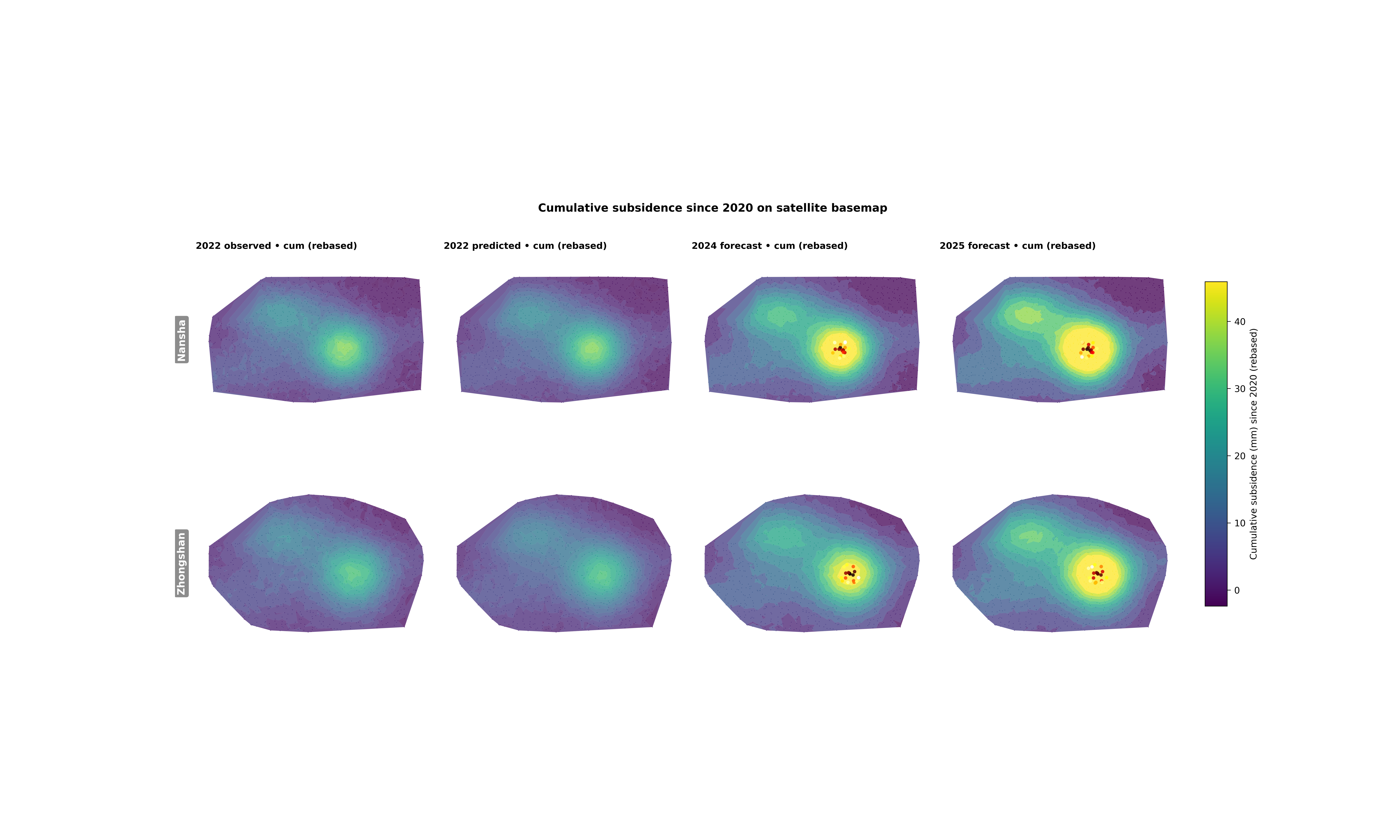
Step 6c - Display the rendered figure

The backend writes the publication-style figure to disk. We reload it here so the gallery page shows the exact final output that a workflow would produce.

img = mpimg.imread(str(out_base) + ".png")

fig, ax = plt.subplots(figsize=(12.0, 7.2))
ax.imshow(img)
ax.axis("off")

(np.float64(-0.5), np.float64(8991.5), np.float64(3685.5), np.float64(-0.5))

Step 6d - Summarize the panels numerically

A gallery page becomes stronger when it teaches both visual and numerical reading.

Here we compute a compact table of median cumulative values for each panel. This helps the reader connect what the eye sees to a simple quantitative summary.

def _city_year_summary(
    city: str,
    val_df: pd.DataFrame,
    fut_df: pd.DataFrame,
) -> pd.DataFrame:
    val = val_df.sort_values(["sample_idx", "coord_t"]).copy()
    fut = fut_df.sort_values(["sample_idx", "coord_t"]).copy()

    val["cum_actual"] = (
        val["subsidence_actual"]
        - val.groupby("sample_idx")["subsidence_actual"].transform(
            "first"
        )
    )

    comb = pd.concat(
        [
            val[
                [
                    "sample_idx",
                    "coord_t",
                    "coord_x",
                    "coord_y",
                    "subsidence_q50",
                ]
            ].copy(),
            fut[
                [
                    "sample_idx",
                    "coord_t",
                    "coord_x",
                    "coord_y",
                    "subsidence_q50",
                ]
            ].copy(),
        ],
        ignore_index=True,
    )
    comb = comb.sort_values(["sample_idx", "coord_t"]).copy()
    comb["cum_pred"] = (
        comb["subsidence_q50"]
        - comb.groupby("sample_idx")["subsidence_q50"].transform(
            "first"
        )
    )

    rows = []
    rows.append(
        {
            "city": city,
            "panel": "2022 observed",
            "median_cumulative": float(
                val.loc[val["coord_t"].eq(2022), "cum_actual"].median()
            ),
        }
    )
    rows.append(
        {
            "city": city,
            "panel": "2022 predicted",
            "median_cumulative": float(
                comb.loc[comb["coord_t"].eq(2022), "cum_pred"].median()
            ),
        }
    )
    for yy in [2024, 2025]:
        rows.append(
            {
                "city": city,
                "panel": f"{yy} forecast",
                "median_cumulative": float(
                    comb.loc[comb["coord_t"].eq(yy), "cum_pred"].median()
                ),
            }
        )

    return pd.DataFrame(rows)


summary = pd.concat(
    [
        _city_year_summary("Nansha", ns_val, ns_future),
        _city_year_summary("Zhongshan", zh_val, zh_future),
    ],
    ignore_index=True,
)

print("\nMedian cumulative subsidence by panel")
print(summary.round(2).to_string(index=False))

Median cumulative subsidence by panel
     city          panel  median_cumulative
   Nansha  2022 observed             6.7300
   Nansha 2022 predicted             6.4900
   Nansha  2024 forecast            10.2200
   Nansha  2025 forecast            12.8400
Zhongshan  2022 observed             7.0900
Zhongshan 2022 predicted             6.8700
Zhongshan  2024 forecast            10.8700
Zhongshan  2025 forecast            13.6600

Next lesson block

Append your interpretation section here:

• Learn how to read the columns

• Learn why the baseline year matters

• Learn what the hotspot overlay adds

• Practical takeaway

• Command-line version

Step 7 - Learn how to read the columns

This figure is easiest to read from left to right.

First column: observed cumulative map

This panel tells you what cumulative subsidence actually looked like in the chosen validation year. It is the spatial reality check.

Second column: predicted cumulative map

This is the model’s cumulative reconstruction for the same year. It answers:

“Did the model learn the broad geography of the cumulative signal?”

Forecast columns

These panels extend the same cumulative logic into the future. Because the color scale is shared across the whole figure, the eye can compare intensification directly across years and across cities.

Step 8 - Learn why the baseline year matters

The plotting script always interprets the map as “cumulative since start_year”.

That sounds small, but it changes the meaning of the figure.

If the input data are already cumulative:

the script rebases them at the first available year.

If the input data are increments or rates:

the script accumulates them.

The scientific meaning is therefore:

• not “absolute deformation ever recorded”,

• but “deformation accumulated since the baseline year used for this analysis”.

That makes start_year a real interpretation choice, not a cosmetic parameter.

Step 9 - Learn what the hotspot overlay adds

The optional hotspot layer is only drawn on forecast panels in the real script. That is useful because it lets the reader see the highest-risk forecast zones without changing the underlying cumulative color field.

In this lesson we colored hotspots by a simple synthetic score, but the script also supports a fixed color overlay. Forecast hotspots are filtered by:

• city

• year

• kind == “forecast”

before being projected to web mercator and drawn.

Step 10 - Practical takeaway

This figure is especially good when you want a spatially intuitive story of accumulation through time.

It is useful for:

• comparing validation-year realism against future evolution,

• comparing the two cities side by side,

• and highlighting where cumulative burden becomes spatially concentrated.

In other words, it is not only a forecast figure. It is a time-accumulation map lesson.

Command-line version

The same figure can be produced from the command line.

The real script accepts:

• --ns-val and --zh-val for the validation CSVs,

• --ns-future and --zh-future for the future CSVs,

• --start-year and --year-val,

• --years-forecast for the forecast columns,

• --subsidence-kind with cumulative | increment | rate,

• --clip and --cmap,

• hotspot options such as --hotspot-csv, --hotspot-field, --hotspot-color, --hotspot-size,

• CRS controls --coords-mode and --utm-epsg,

• and the shared plot text/output options.

Legacy dispatcher:

python -m scripts plot-geo-cumulative \
  --ns-val results/ns_val.csv \
  --zh-val results/zh_val.csv \
  --ns-future results/ns_future.csv \
  --zh-future results/zh_future.csv \
  --start-year 2020 \
  --year-val 2022 \
  --years-forecast 2024 2025 \
  --subsidence-kind cumulative \
  --clip 99 \
  --cmap viridis \
  --hotspot-csv fig6-hotspot-points.csv \
  --hotspot-field delta \
  --out spatial_satellite_cumulative

Modern CLI:

geoprior plot geo-cumulative \
  --ns-val results/ns_val.csv \
  --zh-val results/zh_val.csv \
  --ns-future results/ns_future.csv \
  --zh-future results/zh_future.csv \
  --start-year 2020 \
  --year-val 2022 \
  --years-forecast 2024 2025 \
  --out spatial_satellite_cumulative

The gallery page teaches the figure. The command line reproduces it in a workflow.