
Note
Go to the end to download the full example code.
Physics diagnostics bridge: from evaluate_physics to payload inspection#
This lesson bridges two parts of the GeoPrior documentation:
the diagnostics section, where we ask whether training and evaluation behave sensibly,
and the later physics / model-inspection sections, where we inspect learned fields and mechanistic structure in more detail.
Why this page matters#
Stage-2 training curves can tell us that optimization was stable, but they do not by themselves explain what the physics-informed part of the model actually learned.
That is why GeoPrior exposes a second diagnostic path built around:
GeoPriorSubsNet.evaluate_physics()gather_physics_payload()GeoPriorSubsNet.export_physics_payload()identifiability_diagnostics_from_payload()
The first method evaluates physics consistency directly from model inputs. The payload collector then turns those physics diagnostics into flat 1D arrays suitable for scatter plots, histograms, and summary statistics. The export/load helpers persist the payload for later inspection and figure generation.
What the real helpers do#
evaluate_physics(..., return_maps=True) can expose:
scalar physics diagnostics such as:
loss_cons,loss_gw,loss_prior,epsilon_cons,epsilon_gw,epsilon_priorand optional last-batch maps such as:
R_prior,R_cons,R_gw,K,Ss,tau,tau_prior/tau_closureand thickness fields.
gather_physics_payload(...) then flattens those maps across batches
into arrays such as:
tautau_prior/tau_closureKSsHd(and optionallyH)cons_res_valslog10_taulog10_tau_prior
and also computes summary metrics like:
eps_prior_rmsr2_logtau
with optional closure-consistency metrics when the model exposes a usable scalar kappa value.
What this lesson teaches#
We will:
build a compact synthetic physics payload,
mimic the payload structure returned by the real collector,
inspect the summary metrics and provenance metadata,
plot the main bridge diagnostics: - timescale consistency, - field distributions, - consolidation residual spread,
compute identifiability-style summaries from the payload.
This page uses a synthetic payload so it remains fully executable during the documentation build, but the key names and interpretation are grounded in the real GeoPrior helper contracts.
Imports#
We use the real identifiability payload helper, and we mimic the flat payload layout returned by the real collector.
import numpy as np
import pandas as pd
import matplotlib.pyplot as plt

from geoprior.models.subsidence.payloads import (
    identifiability_diagnostics_from_payload,
)
Step 1 - Build a compact synthetic physics payload#
The real payload collector flattens batch maps into 1D arrays. We mimic that exact style here.
The payload keys are chosen to match the documented contract of
gather_physics_payload(...).
rng = np.random.default_rng(29)

nx = 18
ny = 12

xv = np.linspace(0.0, 12_000.0, nx)
yv = np.linspace(0.0, 8_000.0, ny)
X, Y = np.meshgrid(xv, yv)

coord_x = X.ravel()
coord_y = Y.ravel()
n = coord_x.size

xn = (coord_x - coord_x.min()) / (coord_x.max() - coord_x.min())
yn = (coord_y - coord_y.min()) / (coord_y.max() - coord_y.min())

hotspot = np.exp(
    -(
        ((xn - 0.72) ** 2) / 0.022
        + ((yn - 0.34) ** 2) / 0.032
    )
)
ridge = 0.55 * np.exp(
    -(
        ((xn - 0.28) ** 2) / 0.030
        + ((yn - 0.74) ** 2) / 0.050
    )
)
gradient = 0.40 * xn + 0.22 * (1.0 - yn)

# Physical fields (strictly positive)
K = 10 ** (
    -6.1
    + 0.45 * hotspot
    + 0.10 * gradient
    + rng.normal(0.0, 0.05, size=n)
)
Ss = 10 ** (
    -4.7
    + 0.22 * ridge
    + 0.08 * gradient
    + rng.normal(0.0, 0.04, size=n)
)
Hd = (
    18.0
    + 7.0 * gradient
    + 3.0 * ridge
    + rng.normal(0.0, 0.6, size=n)
)
H = Hd * 1.35

# Effective timescales
kappa_b = 1.0
tau_prior = (Hd ** 2) * Ss / (np.pi**2 * kappa_b * K)
tau = tau_prior * np.exp(rng.normal(0.0, 0.22, size=n))

# Residual-like values
cons_res_vals = rng.normal(0.0, 0.018, size=n)
cons_res_scaled = cons_res_vals / np.maximum(
    np.std(cons_res_vals),
    1e-8,
)
cons_scale = np.full(n, np.std(cons_res_vals))

payload = {
    "tau": tau.astype(np.float32),
    "tau_prior": tau_prior.astype(np.float32),
    "tau_closure": tau_prior.astype(np.float32),
    "K": K.astype(np.float32),
    "Ss": Ss.astype(np.float32),
    "Hd": Hd.astype(np.float32),
    "H": H.astype(np.float32),
    "cons_res_vals": cons_res_vals.astype(np.float32),
    "cons_res_scaled": cons_res_scaled.astype(np.float32),
    "cons_scale": cons_scale.astype(np.float32),
    "log10_tau": np.log10(np.clip(tau, 1e-12, None)).astype(np.float32),
    "log10_tau_prior": np.log10(
        np.clip(tau_prior, 1e-12, None)
    ).astype(np.float32),
}

payload["metrics"] = {
    "eps_prior_rms": float(
        np.sqrt(
            np.mean(
                (
                    np.log(np.clip(payload["tau"], 1e-12, None))
                    - np.log(np.clip(payload["tau_prior"], 1e-12, None))
                )
                ** 2
            )
        )
    ),
    "r2_logtau": float(
        np.corrcoef(
            payload["log10_tau_prior"],
            payload["log10_tau"],
        )[0, 1]
        ** 2
    ),
    "eps_cons_scaled_rms": float(
        np.sqrt(np.mean(payload["cons_res_scaled"] ** 2))
    ),
}

print("Payload keys:")
print(sorted(payload.keys()))

print("")
print("Payload metrics")
print(payload["metrics"])
Payload keys:
['H', 'Hd', 'K', 'Ss', 'cons_res_scaled', 'cons_res_vals', 'cons_scale', 'log10_tau', 'log10_tau_prior', 'metrics', 'tau', 'tau_closure', 'tau_prior']

Payload metrics
{'eps_prior_rms': 0.2198101133108139, 'r2_logtau': 0.52125611135948, 'eps_cons_scaled_rms': 1.0025092363357544}
Step 2 - Build lightweight provenance metadata#
The real export path pairs the payload with metadata from
default_meta_from_model(...). That metadata records the model
name, active PDE modes, kappa interpretation, unit conventions, and
the tau-closure formula used for interpretation.
meta = {
    "model_name": "GeoPriorSubsNet",
    "pde_modes_active": ["consolidation", "gw_flow"],
    "kappa_mode": "kb",
    "kappa_value": 1.0,
    "time_units": "year",
    "time_coord_units": "year",
    "units": {
        "H": "m",
        "Hd": "m",
        "Ss": "1/m",
        "K": "m/s",
        "tau": "s",
        "tau_prior": "s",
        "cons_res_vals": "m/s",
        "kappa": "dimensionless",
    },
    "tau_closure_formula": "Hd^2 * Ss / (pi^2 * kappa_b * K)",
}

print("")
print("Metadata")
for k, v in meta.items():
    print(f"{k}: {v}")
Metadata
model_name: GeoPriorSubsNet
pde_modes_active: ['consolidation', 'gw_flow']
kappa_mode: kb
kappa_value: 1.0
time_units: year
time_coord_units: year
units: {'H': 'm', 'Hd': 'm', 'Ss': '1/m', 'K': 'm/s', 'tau': 's', 'tau_prior': 's', 'cons_res_vals': 'm/s', 'kappa': 'dimensionless'}
tau_closure_formula: Hd^2 * Ss / (pi^2 * kappa_b * K)
Why metadata matters#
Physics payloads are easy to misread if the units or closure conventions are unclear.
This is why the real export helper saves lightweight provenance along with the payload, rather than only the raw arrays.
Step 3 - Build a flat inspection table#
In practice, users often move from the payload dict to a DataFrame for quick inspection and plotting.
diag_df = pd.DataFrame(
    {
        "coord_x": coord_x,
        "coord_y": coord_y,
        "tau": payload["tau"],
        "tau_prior": payload["tau_prior"],
        "K": payload["K"],
        "Ss": payload["Ss"],
        "Hd": payload["Hd"],
        "cons_res_vals": payload["cons_res_vals"],
        "log10_tau": payload["log10_tau"],
        "log10_tau_prior": payload["log10_tau_prior"],
    }
)

print("")
print("Inspection DataFrame head")
print(diag_df.head(8).to_string(index=False))
Inspection DataFrame head
    coord_x  coord_y         tau   tau_prior            K       Ss        Hd  cons_res_vals  log10_tau  log10_tau_prior
   0.000000      0.0  637.243958 1039.790283 7.987420e-07 0.000021 19.843439       0.032950   2.804306         3.016946
 705.882353      0.0  742.090210 1033.966675 8.449849e-07 0.000022 19.812466      -0.032674   2.870457         3.014507
1411.764706      0.0  964.747070  995.014221 8.287936e-07 0.000021 19.743221       0.006166   2.984413         2.997829
2117.647059      0.0 1397.302124 1123.380249 8.330295e-07 0.000020 21.231216       0.005739   3.145290         3.050527
2823.529412      0.0 1074.542358  991.478455 8.600879e-07 0.000021 19.954697       0.000175   3.031224         2.996283
3529.411765      0.0 1022.096741  948.421570 8.365316e-07 0.000021 19.224514      -0.005834   3.009492         2.977001
4235.294118      0.0 1398.885254  913.120300 8.932857e-07 0.000019 20.331606      -0.027187   3.145782         2.960528
4941.176471      0.0  661.147461  917.913757 8.633515e-07 0.000020 19.781975      -0.027740   2.820298         2.962802
Step 4 - Plot timescale consistency#
This is the most important bridge figure.
It answers:
does the learned effective timescale
taubroadly agree with the closure timescaletau_prior?
The payload collector itself already summarizes this with
eps_prior_rms and r2_logtau. The scatter plot shows the same
relationship visually.
fig, ax = plt.subplots(figsize=(6.8, 6.2))

ax.scatter(
    diag_df["log10_tau_prior"],
    diag_df["log10_tau"],
    s=20,
)

lo = float(
    min(
        diag_df["log10_tau_prior"].min(),
        diag_df["log10_tau"].min(),
    )
)
hi = float(
    max(
        diag_df["log10_tau_prior"].max(),
        diag_df["log10_tau"].max(),
    )
)

ax.plot([lo, hi], [lo, hi], linestyle="--", linewidth=1.5)
ax.set_xlabel("log10(tau_prior)")
ax.set_ylabel("log10(tau)")
ax.set_title("Timescale consistency")
ax.grid(True, linestyle=":", alpha=0.6)

plt.tight_layout()
plt.show()
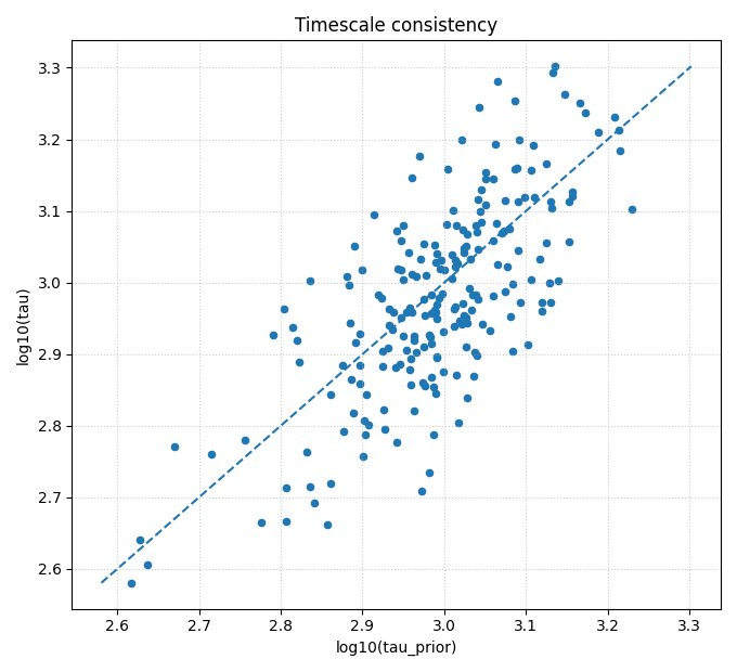
How to read this plot#
Points near the diagonal indicate agreement between:
the learned effective timescale,
and the closure-implied timescale.
A broad but coherent cloud is often acceptable.
A strong systematic shift away from the diagonal can indicate:
closure mismatch,
unit mismatch,
or a regime where the learned fields satisfy the data but violate the intended timescale structure.
Step 5 - Plot field distributions#
The flat payload is ideal for histograms. This is one reason the real collector returns 1D arrays rather than only last-batch maps. It is explicitly designed for scatter plots, histograms, and summary stats.
fig, axes = plt.subplots(1, 3, figsize=(12.0, 4.1))

axes[0].hist(np.log10(diag_df["K"]), bins=20)
axes[0].set_xlabel("log10(K)")
axes[0].set_ylabel("Count")
axes[0].set_title("Hydraulic conductivity")

axes[1].hist(np.log10(diag_df["Ss"]), bins=20)
axes[1].set_xlabel("log10(Ss)")
axes[1].set_ylabel("Count")
axes[1].set_title("Specific storage")

axes[2].hist(diag_df["Hd"], bins=20)
axes[2].set_xlabel("Hd")
axes[2].set_ylabel("Count")
axes[2].set_title("Drainage thickness")

for ax in axes:
    ax.grid(True, linestyle=":", alpha=0.5)

plt.tight_layout()
plt.show()
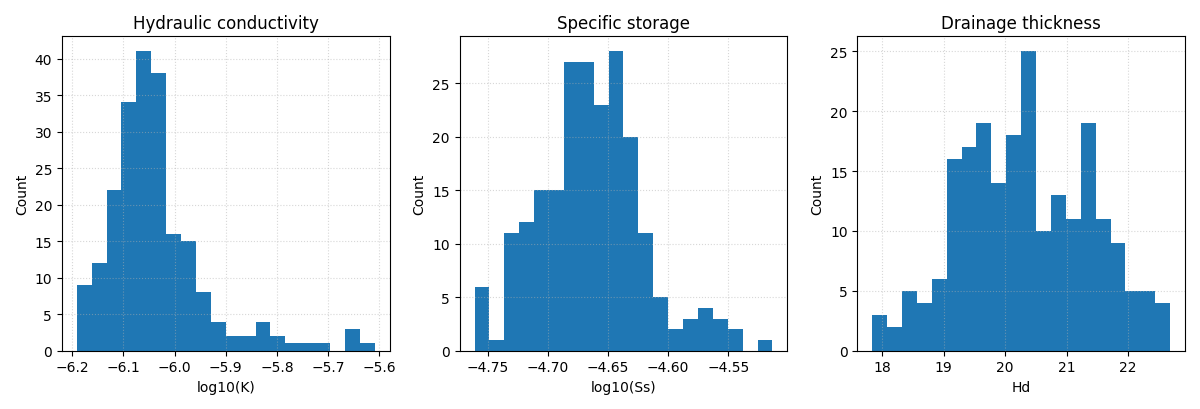
Why these distributions matter#
Before users interpret map-level physics figures, they should first inspect the raw field distributions.
This helps answer:
are the learned fields finite and plausible?
are they concentrated in a narrow range or strongly spread?
do they show suspicious clipping or extreme tails?
Step 6 - Plot consolidation residual spread#
The payload also carries cons_res_vals and can optionally carry
scaled residuals. These are useful bridge diagnostics because they
connect:
the Stage-2 epsilon / loss curves,
and the later spatial physics figures.
fig, axes = plt.subplots(1, 2, figsize=(10.6, 4.1))

axes[0].hist(diag_df["cons_res_vals"], bins=24)
axes[0].set_xlabel("cons_res_vals")
axes[0].set_ylabel("Count")
axes[0].set_title("Consolidation residual distribution")
axes[0].grid(True, linestyle=":", alpha=0.5)

axes[1].scatter(
    diag_df["coord_x"],
    diag_df["coord_y"],
    c=diag_df["cons_res_vals"],
    s=24,
)
axes[1].set_xlabel("coord_x")
axes[1].set_ylabel("coord_y")
axes[1].set_title("Residual pattern in space")
axes[1].grid(True, linestyle=":", alpha=0.5)

plt.tight_layout()
plt.show()
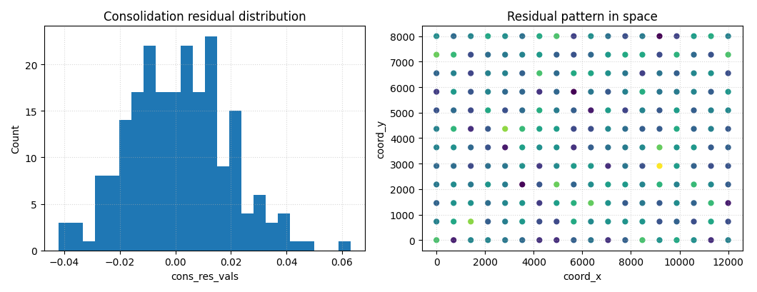
How to read the residual panels#
Histogram#
A residual distribution centered near zero with moderate spread is usually easier to trust than one with a large shift or extreme tails.
Spatial scatter#
Even without a formal map utility, a simple spatial scatter is enough to reveal whether large residuals cluster in one region.
That kind of clustering often motivates the later, more specialized physics-map pages.
Step 7 - Compute identifiability-style diagnostics#
The payload module also provides an explicit helper for synthetic
identifiability analysis:
identifiability_diagnostics_from_payload(...).
It summarizes:
relative error in tau,
closure log-residual,
log-offsets of K, Ss, and Hd versus true and prior values.
tau_true = float(np.median(payload["tau"]))
K_true = float(np.median(payload["K"]))
Ss_true = float(np.median(payload["Ss"]))
Hd_true = float(np.median(payload["Hd"]))

# Slightly different "prior" values for demonstration.
K_prior = K_true * 0.85
Ss_prior = Ss_true * 1.10
Hd_prior = Hd_true * 0.95

ident = identifiability_diagnostics_from_payload(
    payload,
    tau_true=tau_true,
    K_true=K_true,
    Ss_true=Ss_true,
    Hd_true=Hd_true,
    K_prior=K_prior,
    Ss_prior=Ss_prior,
    Hd_prior=Hd_prior,
)

print("")
print("Identifiability diagnostics")
print(ident)
Identifiability diagnostics
{'tau_rel_error': {'mean': 0.25018756904290457, 'std': 0.2210769271338095, 'q50': 0.18871058765321386, 'q75': 0.35665904543234883, 'q90': 0.5228325222484639, 'q95': 0.683088429510347}, 'closure_log_resid': {'mean': 0.03655655557653968, 'std': 0.23825474978879382, 'q50': 0.04438027640654951, 'q75': 0.17445646408851134, 'q90': 0.32793751713727515, 'q95': 0.3946892124192971}, 'offsets': {'vs_true': {'delta_K': {'mean': 0.03819718679708197, 'std': 0.2267048409488427, 'q50': -1.639305766687471e-07, 'q75': 0.1042537625590585, 'q90': 0.26360858012960353, 'q95': 0.5152721508909335}, 'delta_Ss': {'mean': -0.0006256768178957192, 'std': 0.10069134160640923, 'q50': -7.932463841342496e-08, 'q75': 0.05171015811850044, 'q90': 0.11098079454196164, 'q95': 0.1972537370990728}, 'delta_Hd': {'mean': 0.0007978356292350178, 'std': 0.0515580902850574, 'q50': -2.2123230802861826e-08, 'q75': 0.04147887330814648, 'q90': 0.06878093111456329, 'q95': 0.08505455071140844}}, 'vs_prior': {'delta_K': {'mean': 0.20071611629485708, 'std': 0.2267048409488427, 'q50': 0.16251876556719846, 'q75': 0.2667726920568336, 'q90': 0.42612750962737866, 'q95': 0.6777910803887086}, 'delta_Ss': {'mean': -0.0959358566222196, 'std': 0.10069134160640923, 'q50': -0.0953102591289623, 'q75': -0.04360002168582344, 'q90': 0.015670614737637756, 'q95': 0.10194355729474891}, 'delta_Hd': {'mean': 0.052091130016785614, 'std': 0.0515580902850574, 'q50': 0.05129327226431979, 'q75': 0.09277216769569707, 'q90': 0.12007422550211388, 'q95': 0.13634784509895903}}}}
Why this matters#
This helper is not just for SM3-style synthetic studies.
In the documentation flow, it is also useful as a bridge because it shows how a flat payload can support:
consistency checks,
offset diagnostics,
and identifiability-oriented summaries,
before users move to the later, more specialized figure-generation pages.
Step 8 - Build a compact summary table#
A diagnostics bridge page should end with a small summary the user could plausibly print or export.
summary = pd.DataFrame(
    [
        {
            "metric": "eps_prior_rms",
            "value": float(payload["metrics"]["eps_prior_rms"]),
        },
        {
            "metric": "r2_logtau",
            "value": float(payload["metrics"]["r2_logtau"]),
        },
        {
            "metric": "eps_cons_scaled_rms",
            "value": float(payload["metrics"]["eps_cons_scaled_rms"]),
        },
        {
            "metric": "median_log10_K",
            "value": float(np.median(np.log10(payload["K"]))),
        },
        {
            "metric": "median_log10_Ss",
            "value": float(np.median(np.log10(payload["Ss"]))),
        },
        {
            "metric": "median_Hd",
            "value": float(np.median(payload["Hd"])),
        },
    ]
)

print("")
print("Physics payload summary")
print(summary.to_string(index=False))
Physics payload summary
             metric     value
      eps_prior_rms  0.219810
          r2_logtau  0.521256
eps_cons_scaled_rms  1.002509
     median_log10_K -6.051237
    median_log10_Ss -4.663055
          median_Hd 20.293217
Step 9 - Practical interpretation guide#
This bridge page should be read in the following order:
inspect the summary metrics,
inspect timescale consistency,
inspect field distributions,
inspect residual spread,
then move on to dedicated physics-map or identifiability pages.
That order matters because it helps users distinguish:
a model that is numerically stable but physically incoherent,
from one that is both stable and mechanistically interpretable.
Final takeaway#
This page sits between diagnostics and the later physics sections for a reason.
It shows how to move from:
Stage-2 style residual and loss summaries,
to flat physics payloads,
to interpretable mechanistic diagnostics.
In GeoPrior, that bridge is built by:
evaluate_physics(...)gather_physics_payload(...)export_physics_payload(...)identifiability_diagnostics_from_payload(...)
Understanding that bridge makes the later model-inspection and figure-generation pages much easier to read.
Total running time of the script: (0 minutes 0.720 seconds)