
Note
Go to the end to download the full example code.
Build ablation tables from sensitivity records#
This example teaches you how to use GeoPrior’s
build-ablation-table utility.
Unlike the figure-generation scripts, this command does not start from a plotting function. It starts from raw or semi-processed ablation records and turns them into tidy, reusable analysis tables.
Why this matters#
Ablation experiments are only useful if their outputs can be compared, filtered, exported, and reused downstream.
This builder helps turn a folder of
ablation_record*.jsonl files into:
one tidy ablation table,
one optional best-per-city table,
optional grouped S6 lambda grids,
optional grouped S7 toggle summaries.
That makes it a strong first lesson for the
tables_and_summaries section.
Imports#
We call the real production entrypoint from the project code. Then we read the generated tables back in and build one compact visual preview for the lesson page.
from __future__ import annotations

import json
import tempfile
from pathlib import Path

import matplotlib.pyplot as plt
import numpy as np
import pandas as pd

from geoprior.scripts.build_ablation_table import (
    build_ablation_table_main,
)
Build a compact synthetic ablation study#
The real script expects ablation records such as
ablation_record*.jsonl. Each record is a dictionary with
run metadata and metrics.
For the lesson, we create a small synthetic study with:
two cities,
two physics buckets,
a lambda_prior × lambda_cons grid,
overall metrics,
and per-horizon metrics.
We also include the toggle-style fields used by the script’s S7 grouped summary logic:
lambda_smooth
lambda_bounds
lambda_mv
lambda_q
use_effective_h
kappa_mode
hd_factor
lambda_prior_vals = [0.0, 0.1, 0.3, 1.0]
lambda_cons_vals = [0.0, 0.1, 0.3, 1.0]

rows: list[dict[str, object]] = []
counter = 0

for city in ["Nansha", "Zhongshan"]:
    city_shift = 0.0 if city == "Nansha" else 0.55

    for pde_mode in ["both", "none"]:
        phys_penalty = 0.0 if pde_mode == "both" else 1.25

        for lp in lambda_prior_vals:
            for lc in lambda_cons_vals:
                counter += 1

                log_lp = np.log10(lp + 0.12)
                log_lc = np.log10(lc + 0.12)

                mae = (
                    4.8
                    + city_shift
                    + phys_penalty
                    + 1.8 * (log_lp + 0.22) ** 2
                    + 1.1 * (log_lc + 0.18) ** 2
                )

                rmse = mae * 1.18
                mse = rmse**2

                epsilon_prior = (
                    0.26
                    + 0.04 * city_shift
                    + 0.08 * (log_lp + 0.22) ** 2
                    + 0.03 * (log_lc + 0.10) ** 2
                    + 0.08 * (pde_mode == "none")
                )

                epsilon_cons = (
                    0.22
                    + 0.04 * city_shift
                    + 0.03 * (log_lp + 0.08) ** 2
                    + 0.09 * (log_lc + 0.25) ** 2
                    + 0.08 * (pde_mode == "none")
                )

                coverage80 = np.clip(
                    0.95
                    - 0.08 * epsilon_prior
                    - 0.06 * epsilon_cons,
                    0.65,
                    0.98,
                )

                sharpness80 = (
                    15.0
                    + 3.5 * (log_lp + 0.18) ** 2
                    + 5.5 * (log_lc + 0.25) ** 2
                    + 1.0 * (pde_mode == "none")
                )

                r2 = np.clip(
                    0.95
                    - 0.050 * mae
                    - 0.004 * sharpness80,
                    0.10,
                    0.96,
                )

                use_effective_h = bool(
                    city == "Zhongshan" or lp >= 0.3
                )
                hd_factor = 0.6 if use_effective_h else 1.0
                kappa_mode = "bar" if city == "Nansha" else "kb"

                row = {
                    "timestamp": (
                        f"2026-03-28T12:{counter:02d}:00"
                    ),
                    "city": city,
                    "model": "GeoPriorSubsNet",
                    "pde_mode": pde_mode,
                    "use_effective_h": use_effective_h,
                    "kappa_mode": kappa_mode,
                    "hd_factor": float(hd_factor),
                    "lambda_prior": float(lp),
                    "lambda_cons": float(lc),
                    "lambda_gw": (
                        0.20 if pde_mode == "both" else 0.0
                    ),
                    "lambda_smooth": 0.40 if lp >= 0.3 else 0.0,
                    "lambda_mv": 0.08 if lp >= 0.1 else 0.0,
                    "lambda_bounds": 0.05 if lc >= 0.1 else 0.0,
                    "lambda_q": 0.03 if lc >= 0.3 else 0.0,
                    "mae": float(mae),
                    "rmse": float(rmse),
                    "mse": float(mse),
                    "r2": float(r2),
                    "coverage80": float(coverage80),
                    "sharpness80": float(sharpness80),
                    "epsilon_prior": float(epsilon_prior),
                    "epsilon_cons": float(epsilon_cons),
                    "units": {"subs_metrics_unit": "mm"},
                    "per_horizon_mae": {
                        "H1": float(mae * 0.86),
                        "H2": float(mae),
                        "H3": float(mae * 1.15),
                    },
                    "per_horizon_r2": {
                        "H1": float(min(0.99, r2 + 0.04)),
                        "H2": float(r2),
                        "H3": float(max(0.0, r2 - 0.05)),
                    },
                }
                rows.append(row)

print(f"Number of synthetic records: {len(rows)}")
print("")
print("Example record")
print(json.dumps(rows[0], indent=2))
Number of synthetic records: 64

Example record
{
  "timestamp": "2026-03-28T12:01:00",
  "city": "Nansha",
  "model": "GeoPriorSubsNet",
  "pde_mode": "both",
  "use_effective_h": false,
  "kappa_mode": "bar",
  "hd_factor": 1.0,
  "lambda_prior": 0.0,
  "lambda_cons": 0.0,
  "lambda_gw": 0.2,
  "lambda_smooth": 0.0,
  "lambda_mv": 0.0,
  "lambda_bounds": 0.0,
  "lambda_q": 0.0,
  "mae": 6.287758135432752,
  "rmse": 7.419554599810647,
  "mse": 55.049790459571334,
  "r2": 0.5580287676470639,
  "coverage80": 0.9075371302077502,
  "sharpness80": 19.395831395324617,
  "epsilon_prior": 0.31950405687650674,
  "epsilon_cons": 0.2817090873688203,
  "units": {
    "subs_metrics_unit": "mm"
  },
  "per_horizon_mae": {
    "H1": 5.407471996472167,
    "H2": 6.287758135432752,
    "H3": 7.230921855747664
  },
  "per_horizon_r2": {
    "H1": 0.5980287676470639,
    "H2": 0.5580287676470639,
    "H3": 0.5080287676470638
  }
}
Write the synthetic JSONL file#
The production command reads ablation records from files, so we follow that same workflow here.
tmp_dir = Path(
    tempfile.mkdtemp(prefix="gp_sg_ablation_table_")
)
jsonl_path = tmp_dir / "ablation_record.synthetic.jsonl"

with jsonl_path.open("w", encoding="utf-8") as f:
    for rec in rows:
        f.write(json.dumps(rec) + "\n")

print("")
print(f"Input JSONL written to: {jsonl_path}")
Input JSONL written to: /tmp/gp_sg_ablation_table_gl6qbufn/ablation_record.synthetic.jsonl
Run the real ablation-table builder#
We ask the script to produce:
the main tidy table,
a best-per-city table,
grouped S6 lambda grids,
and an S7 grouped toggle summary.
We keep the output in CSV/JSON/TXT form for the lesson page.
out_stem = "ablation_table_gallery"

build_ablation_table_main(
    [
        "--input",
        str(jsonl_path),
        "--out-dir",
        str(tmp_dir),
        "--out",
        out_stem,
        "--formats",
        "csv,json,txt",
        "--sort-by",
        "mae",
        "--ascending",
        "auto",
        "--metric-unit",
        "mm",
        "--keep-per-horizon",
        "true",
        "--best-per-city",
        "--group-cols",
        "s6,s7",
        "--s6-metrics",
        "mae,coverage80,sharpness80",
        "--s7-metrics",
        "mae,coverage80,sharpness80",
        "--s7-agg",
        "mean",
    ],
    prog="build-ablation-table",
)
[OK] csv -> /tmp/gp_sg_ablation_table_gl6qbufn/ablation_table_gallery.csv
[OK] json -> /tmp/gp_sg_ablation_table_gl6qbufn/ablation_table_gallery.json
[OK] txt -> /tmp/gp_sg_ablation_table_gl6qbufn/ablation_table_gallery.txt
[OK] best/city -> /tmp/gp_sg_ablation_table_gl6qbufn/ablation_table_gallery__best_per_city.csv
[OK] csv -> /tmp/gp_sg_ablation_table_gl6qbufn/ablation_table_gallery__S6__mae__Nansha__both.csv
[OK] json -> /tmp/gp_sg_ablation_table_gl6qbufn/ablation_table_gallery__S6__mae__Nansha__both.json
[OK] txt -> /tmp/gp_sg_ablation_table_gl6qbufn/ablation_table_gallery__S6__mae__Nansha__both.txt
[OK] csv -> /tmp/gp_sg_ablation_table_gl6qbufn/ablation_table_gallery__S6__coverage80__Nansha__both.csv
[OK] json -> /tmp/gp_sg_ablation_table_gl6qbufn/ablation_table_gallery__S6__coverage80__Nansha__both.json
[OK] txt -> /tmp/gp_sg_ablation_table_gl6qbufn/ablation_table_gallery__S6__coverage80__Nansha__both.txt
[OK] csv -> /tmp/gp_sg_ablation_table_gl6qbufn/ablation_table_gallery__S6__sharpness80__Nansha__both.csv
[OK] json -> /tmp/gp_sg_ablation_table_gl6qbufn/ablation_table_gallery__S6__sharpness80__Nansha__both.json
[OK] txt -> /tmp/gp_sg_ablation_table_gl6qbufn/ablation_table_gallery__S6__sharpness80__Nansha__both.txt
[OK] csv -> /tmp/gp_sg_ablation_table_gl6qbufn/ablation_table_gallery__S6__mae__Nansha__none.csv
[OK] json -> /tmp/gp_sg_ablation_table_gl6qbufn/ablation_table_gallery__S6__mae__Nansha__none.json
[OK] txt -> /tmp/gp_sg_ablation_table_gl6qbufn/ablation_table_gallery__S6__mae__Nansha__none.txt
[OK] csv -> /tmp/gp_sg_ablation_table_gl6qbufn/ablation_table_gallery__S6__coverage80__Nansha__none.csv
[OK] json -> /tmp/gp_sg_ablation_table_gl6qbufn/ablation_table_gallery__S6__coverage80__Nansha__none.json
[OK] txt -> /tmp/gp_sg_ablation_table_gl6qbufn/ablation_table_gallery__S6__coverage80__Nansha__none.txt
[OK] csv -> /tmp/gp_sg_ablation_table_gl6qbufn/ablation_table_gallery__S6__sharpness80__Nansha__none.csv
[OK] json -> /tmp/gp_sg_ablation_table_gl6qbufn/ablation_table_gallery__S6__sharpness80__Nansha__none.json
[OK] txt -> /tmp/gp_sg_ablation_table_gl6qbufn/ablation_table_gallery__S6__sharpness80__Nansha__none.txt
[OK] csv -> /tmp/gp_sg_ablation_table_gl6qbufn/ablation_table_gallery__S6__mae__Zhongshan__both.csv
[OK] json -> /tmp/gp_sg_ablation_table_gl6qbufn/ablation_table_gallery__S6__mae__Zhongshan__both.json
[OK] txt -> /tmp/gp_sg_ablation_table_gl6qbufn/ablation_table_gallery__S6__mae__Zhongshan__both.txt
[OK] csv -> /tmp/gp_sg_ablation_table_gl6qbufn/ablation_table_gallery__S6__coverage80__Zhongshan__both.csv
[OK] json -> /tmp/gp_sg_ablation_table_gl6qbufn/ablation_table_gallery__S6__coverage80__Zhongshan__both.json
[OK] txt -> /tmp/gp_sg_ablation_table_gl6qbufn/ablation_table_gallery__S6__coverage80__Zhongshan__both.txt
[OK] csv -> /tmp/gp_sg_ablation_table_gl6qbufn/ablation_table_gallery__S6__sharpness80__Zhongshan__both.csv
[OK] json -> /tmp/gp_sg_ablation_table_gl6qbufn/ablation_table_gallery__S6__sharpness80__Zhongshan__both.json
[OK] txt -> /tmp/gp_sg_ablation_table_gl6qbufn/ablation_table_gallery__S6__sharpness80__Zhongshan__both.txt
[OK] csv -> /tmp/gp_sg_ablation_table_gl6qbufn/ablation_table_gallery__S6__mae__Zhongshan__none.csv
[OK] json -> /tmp/gp_sg_ablation_table_gl6qbufn/ablation_table_gallery__S6__mae__Zhongshan__none.json
[OK] txt -> /tmp/gp_sg_ablation_table_gl6qbufn/ablation_table_gallery__S6__mae__Zhongshan__none.txt
[OK] csv -> /tmp/gp_sg_ablation_table_gl6qbufn/ablation_table_gallery__S6__coverage80__Zhongshan__none.csv
[OK] json -> /tmp/gp_sg_ablation_table_gl6qbufn/ablation_table_gallery__S6__coverage80__Zhongshan__none.json
[OK] txt -> /tmp/gp_sg_ablation_table_gl6qbufn/ablation_table_gallery__S6__coverage80__Zhongshan__none.txt
[OK] csv -> /tmp/gp_sg_ablation_table_gl6qbufn/ablation_table_gallery__S6__sharpness80__Zhongshan__none.csv
[OK] json -> /tmp/gp_sg_ablation_table_gl6qbufn/ablation_table_gallery__S6__sharpness80__Zhongshan__none.json
[OK] txt -> /tmp/gp_sg_ablation_table_gl6qbufn/ablation_table_gallery__S6__sharpness80__Zhongshan__none.txt
[OK] csv -> /tmp/gp_sg_ablation_table_gl6qbufn/ablation_table_gallery__S7.csv
[OK] json -> /tmp/gp_sg_ablation_table_gl6qbufn/ablation_table_gallery__S7.json
[OK] txt -> /tmp/gp_sg_ablation_table_gl6qbufn/ablation_table_gallery__S7.txt
Inspect the produced files#
The command writes multiple outputs. For the lesson, we list the main ones so the user sees the artifact family clearly.
written = sorted(tmp_dir.glob("ablation_table_gallery*"))

print("")
print("Written files")
for p in written:
    print(" -", p.name)
Written files
 - ablation_table_gallery.csv
 - ablation_table_gallery.json
 - ablation_table_gallery.txt
 - ablation_table_gallery__S6__coverage80__Nansha__both.csv
 - ablation_table_gallery__S6__coverage80__Nansha__both.json
 - ablation_table_gallery__S6__coverage80__Nansha__both.txt
 - ablation_table_gallery__S6__coverage80__Nansha__none.csv
 - ablation_table_gallery__S6__coverage80__Nansha__none.json
 - ablation_table_gallery__S6__coverage80__Nansha__none.txt
 - ablation_table_gallery__S6__coverage80__Zhongshan__both.csv
 - ablation_table_gallery__S6__coverage80__Zhongshan__both.json
 - ablation_table_gallery__S6__coverage80__Zhongshan__both.txt
 - ablation_table_gallery__S6__coverage80__Zhongshan__none.csv
 - ablation_table_gallery__S6__coverage80__Zhongshan__none.json
 - ablation_table_gallery__S6__coverage80__Zhongshan__none.txt
 - ablation_table_gallery__S6__mae__Nansha__both.csv
 - ablation_table_gallery__S6__mae__Nansha__both.json
 - ablation_table_gallery__S6__mae__Nansha__both.txt
 - ablation_table_gallery__S6__mae__Nansha__none.csv
 - ablation_table_gallery__S6__mae__Nansha__none.json
 - ablation_table_gallery__S6__mae__Nansha__none.txt
 - ablation_table_gallery__S6__mae__Zhongshan__both.csv
 - ablation_table_gallery__S6__mae__Zhongshan__both.json
 - ablation_table_gallery__S6__mae__Zhongshan__both.txt
 - ablation_table_gallery__S6__mae__Zhongshan__none.csv
 - ablation_table_gallery__S6__mae__Zhongshan__none.json
 - ablation_table_gallery__S6__mae__Zhongshan__none.txt
 - ablation_table_gallery__S6__sharpness80__Nansha__both.csv
 - ablation_table_gallery__S6__sharpness80__Nansha__both.json
 - ablation_table_gallery__S6__sharpness80__Nansha__both.txt
 - ablation_table_gallery__S6__sharpness80__Nansha__none.csv
 - ablation_table_gallery__S6__sharpness80__Nansha__none.json
 - ablation_table_gallery__S6__sharpness80__Nansha__none.txt
 - ablation_table_gallery__S6__sharpness80__Zhongshan__both.csv
 - ablation_table_gallery__S6__sharpness80__Zhongshan__both.json
 - ablation_table_gallery__S6__sharpness80__Zhongshan__both.txt
 - ablation_table_gallery__S6__sharpness80__Zhongshan__none.csv
 - ablation_table_gallery__S6__sharpness80__Zhongshan__none.json
 - ablation_table_gallery__S6__sharpness80__Zhongshan__none.txt
 - ablation_table_gallery__S7.csv
 - ablation_table_gallery__S7.json
 - ablation_table_gallery__S7.txt
 - ablation_table_gallery__best_per_city.csv
Read the main table and the grouped outputs#
The main table is the tidy run-level export. S6 is the lambda grid summary. S7 is the grouped toggle summary. The best-per-city table is a very useful quick summary.
main_csv = tmp_dir / "ablation_table_gallery.csv"
best_csv = (
    tmp_dir / "ablation_table_gallery__best_per_city.csv"
)
s6_csv = (
    tmp_dir
    / "ablation_table_gallery__S6__mae__Nansha__both.csv"
)
s7_csv = tmp_dir / "ablation_table_gallery__S7.csv"

tab = pd.read_csv(main_csv)
best = pd.read_csv(best_csv)
s6 = pd.read_csv(s6_csv)
s7 = pd.read_csv(s7_csv)

print("")
print("Main tidy table")
print(tab.head(8).to_string(index=False))

print("")
print("Best per city")
print(best.to_string(index=False))

print("")
print("S7 grouped summary")
print(s7.head(12).to_string(index=False))
Main tidy table
          timestamp   city           model pde_mode  use_effective_h kappa_mode  hd_factor  lambda_cons  lambda_gw  lambda_prior  lambda_smooth  lambda_mv  lambda_bounds  lambda_q    mae   rmse     mse     r2  coverage80  sharpness80  epsilon_prior  epsilon_cons  per_horizon_mae.H1  per_horizon_mae.H2  per_horizon_mae.H3  per_horizon_r2.H1  per_horizon_r2.H2  per_horizon_r2.H3
2026-03-28T12:11:00 Nansha GeoPriorSubsNet     both             True        bar     0.6000       0.3000     0.2000        0.3000         0.4000     0.0800         0.0500    0.0300 4.8868 5.7664 33.2518 0.6448      0.9154      15.2238         0.2643        0.2241              4.2027              4.8868              5.6198             0.6848             0.6448             0.5948
2026-03-28T12:12:00 Nansha GeoPriorSubsNet     both             True        bar     0.6000       1.0000     0.2000        0.3000         0.4000     0.0800         0.0500    0.0300 4.9020 5.7844 33.4591 0.6424      0.9151      15.6279         0.2626        0.2307              4.2157              4.9020              5.6373             0.6824             0.6424             0.5924
2026-03-28T12:15:00 Nansha GeoPriorSubsNet     both             True        bar     0.6000       0.3000     0.2000        1.0000         0.4000     0.0800         0.0500    0.0300 4.9730 5.8682 34.4357 0.6403      0.9152      15.2723         0.2681        0.2219              4.2768              4.9730              5.7190             0.6803             0.6403             0.5903
2026-03-28T12:16:00 Nansha GeoPriorSubsNet     both             True        bar     0.6000       1.0000     0.2000        1.0000         0.4000     0.0800         0.0500    0.0300 4.9883 5.8861 34.6467 0.6379      0.9150      15.6763         0.2665        0.2286              4.2899              4.9883              5.7365             0.6779             0.6379             0.5879
2026-03-28T12:10:00 Nansha GeoPriorSubsNet     both             True        bar     0.6000       0.1000     0.2000        0.3000         0.4000     0.0800         0.0500    0.0000 5.0951 6.0122 36.1470 0.6310      0.9140      16.0491         0.2713        0.2376              4.3818              5.0951              5.8594             0.6710             0.6310             0.5810
2026-03-28T12:14:00 Nansha GeoPriorSubsNet     both             True        bar     0.6000       0.1000     0.2000        1.0000         0.4000     0.0800         0.0500    0.0000 5.1813 6.1140 37.3809 0.6265      0.9139      16.0975         0.2751        0.2355              4.4560              5.1813              5.9586             0.6665             0.6265             0.5765
2026-03-28T12:07:00 Nansha GeoPriorSubsNet     both            False        bar     1.0000       0.3000     0.2000        0.1000         0.0000     0.0800         0.0500    0.0300 5.1872 6.1209 37.4659 0.6271      0.9139      15.8866         0.2776        0.2315              4.4610              5.1872              5.9653             0.6671             0.6271             0.5771
2026-03-28T12:08:00 Nansha GeoPriorSubsNet     both            False        bar     1.0000       1.0000     0.2000        0.1000         0.0000     0.0800         0.0500    0.0300 5.2024 6.1389 37.6860 0.6247      0.9136      16.2907         0.2760        0.2381              4.4741              5.2024              5.9828             0.6647             0.6247             0.5747

Best per city
          timestamp      city           model pde_mode  use_effective_h kappa_mode  hd_factor  lambda_cons  lambda_gw  lambda_prior  lambda_smooth  lambda_mv  lambda_bounds  lambda_q    mae   rmse     mse     r2  coverage80  sharpness80  epsilon_prior  epsilon_cons  per_horizon_mae.H1  per_horizon_mae.H2  per_horizon_mae.H3  per_horizon_r2.H1  per_horizon_r2.H2  per_horizon_r2.H3
2026-03-28T12:11:00    Nansha GeoPriorSubsNet     both             True        bar     0.6000       0.3000     0.2000        0.3000         0.4000     0.0800         0.0500    0.0300 4.8868 5.7664 33.2518 0.6448      0.9154      15.2238         0.2643        0.2241              4.2027              4.8868              5.6198             0.6848             0.6448             0.5948
2026-03-28T12:43:00 Zhongshan GeoPriorSubsNet     both             True         kb     0.6000       0.3000     0.2000        0.3000         0.4000     0.0800         0.0500    0.0300 5.4368 6.4154 41.1578 0.6173      0.9123      15.2238         0.2863        0.2461              4.6757              5.4368              6.2523             0.6573             0.6173             0.5673

S7 grouped summary
  city pde_bucket  use_effective_h kappa_mode  hd_factor smooth_on bounds_on mv_on q_on  n    mae  coverage80  sharpness80
Nansha       both            False        bar     1.0000       off       off   off  off  1 6.2878      0.9075      19.3958
Nansha       both            False        bar     1.0000       off       off    on  off  1 5.7483      0.9101      18.2733
Nansha       both            False        bar     1.0000       off        on   off  off  1 5.9350      0.9099      17.8345
Nansha       both            False        bar     1.0000       off        on   off   on  2 5.7343      0.9112      17.2112
Nansha       both            False        bar     1.0000       off        on    on  off  1 5.3955      0.9125      16.7119
Nansha       both            False        bar     1.0000       off        on    on   on  2 5.1948      0.9138      16.0887
Nansha       both             True        bar     0.6000        on       off    on  off  2 5.4910      0.9115      17.6347
Nansha       both             True        bar     0.6000        on        on    on  off  2 5.1382      0.9140      16.0733
Nansha       both             True        bar     0.6000        on        on    on   on  4 4.9375      0.9152      15.4501
Nansha       none            False        bar     1.0000       off       off   off  off  1 7.5378      0.8963      20.3958
Nansha       none            False        bar     1.0000       off       off    on  off  1 6.9983      0.8989      19.2733
Nansha       none            False        bar     1.0000       off        on   off  off  1 7.1850      0.8987      18.8345
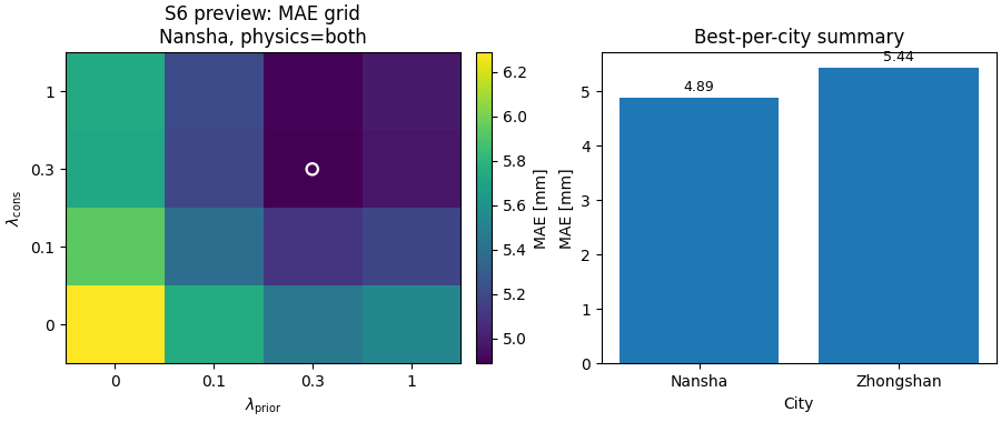
Build one compact visual preview from the generated tables#
This is not part of the production builder itself. It is a teaching aid for the gallery page.
- Left:
an S6 heatmap for MAE in Nansha with physics on.
- Right:
the best-per-city MAE summary.
# Rebuild the S6 matrix from the flat CSV.
lcons = pd.to_numeric(
    s6.iloc[:, 0], errors="coerce"
).to_numpy()
lpris = np.array([float(c) for c in s6.columns[1:]])
heat = s6.iloc[:, 1:].to_numpy(dtype=float)

fig, axes = plt.subplots(
    1,
    2,
    figsize=(9.0, 3.8),
    constrained_layout=True,
)

# S6 heatmap
ax = axes[0]
im = ax.imshow(
    heat,
    origin="lower",
    aspect="auto",
)
ax.set_title("S6 preview: MAE grid\nNansha, physics=both")
ax.set_xlabel(r"$\lambda_{\mathrm{prior}}$")
ax.set_ylabel(r"$\lambda_{\mathrm{cons}}$")
ax.set_xticks(np.arange(len(lpris)))
ax.set_yticks(np.arange(len(lcons)))
ax.set_xticklabels([f"{x:g}" for x in lpris])
ax.set_yticklabels([f"{x:g}" for x in lcons])

# Mark the best cell.
i_best, j_best = np.unravel_index(
    np.nanargmin(heat),
    heat.shape,
)
ax.scatter(
    [j_best],
    [i_best],
    marker="o",
    s=55,
    facecolors="none",
    edgecolors="white",
    linewidths=1.6,
)

cbar = fig.colorbar(im, ax=ax, fraction=0.046, pad=0.04)
cbar.set_label("MAE [mm]")

# Best-per-city bar chart
ax = axes[1]
ax.bar(best["city"], best["mae"])
ax.set_title("Best-per-city summary")
ax.set_ylabel("MAE [mm]")
ax.set_xlabel("City")

for i, v in enumerate(best["mae"].to_numpy(float)):
    ax.text(
        i,
        v + 0.06,
        f"{v:.2f}",
        ha="center",
        va="bottom",
        fontsize=9,
    )
Learn how to read the main table#
The main tidy table is the run-level table.
A useful reading order is:
identify the configuration columns such as city, pde_mode, lambda weights, and identifiability settings;
read the main metrics such as MAE, RMSE, R2, coverage80, and sharpness80;
use the per-horizon columns only when you need to inspect how performance drifts across forecast steps.
In other words:
the main table is the tidy archive,
the grouped tables are the paper-style summaries.
Learn how to read the S6 table#
The S6 output is the lambda-grid summary.
For each city and each physics bucket, the script pivots one metric onto:
rows = lambda_cons
cols = lambda_prior
This is extremely useful because it converts a long run table into a sensitivity surface that can later be:
plotted as a heatmap,
exported to TeX,
or inspected directly in CSV form.
In the preview heatmap above, the white ring marks the best MAE cell in the Nansha + physics-on grid.
Learn how to read the S7 table#
The S7 output is the toggle summary.
Instead of summarizing individual runs, it groups runs by higher-level settings such as:
city,
pde bucket,
use_effective_h,
kappa_mode,
smooth_on,
bounds_on,
mv_on,
q_on.
Then it computes group means and group sizes.
This is useful when the reader is not asking:
“Which exact lambda pair won?”
but instead:
“Do runs with bounds or smoothness tend to behave better on average?”
Why this builder is useful in practice#
This script is a strong bridge between raw experiment logs and later analysis pages.
It helps with three different kinds of work:
quick filtering and ranking of runs,
paper-style grouped summaries,
and downstream figure generation such as S6 sensitivity maps.
That is why it belongs naturally in the
tables_and_summaries gallery rather than in
figure_generation.
Practical takeaway#
A good workflow for ablations is:
run the sensitivity or ablation jobs,
build the tidy ablation table,
inspect best-per-city rows,
inspect S6 lambda grids,
inspect S7 grouped toggle summaries,
only then move on to paper-ready plots.
This order helps separate:
data collection,
tabulation,
and visualization.
Command-line version#
The same lesson can be reproduced from the CLI.
Legacy dispatcher:
python -m scripts build-ablation-table \
  --root results \
  --out table_ablations \
  --formats csv,json,txt \
  --best-per-city \
  --group-cols s6,s7
Paper-friendly TeX export:
python -m scripts build-ablation-table \
  --root results \
  --for-paper \
  --err-metric rmse \
  --keep-r2 \
  --formats csv,tex \
  --out table_ablations_paper
Modern CLI:
geoprior build ablation-table \
  --root results \
  --out table_ablations \
  --group-cols s6,s7
The gallery page teaches the builder. The command line reproduces it in a workflow.
Total running time of the script: (0 minutes 0.376 seconds)