Read forecast reliability with plot_reliability_diagram

This lesson explains how to use geoprior.plot.forecast.plot_reliability_diagram when you want a direct visual answer to a simple question:

Do the forecast probabilities or forecast quantiles behave like they claim?

Why this function matters

A probabilistic forecast is useful only when its probabilities are trustworthy.

That trust can fail in two different ways:

• quantile forecasts may be too narrow or too wide, so a nominal 90th percentile does not really contain about 90 percent of the observations below it,

• probability forecasts may look confident while systematically overpredicting or underpredicting event frequency.

This helper gives one of the clearest first-pass calibration checks in the whole plotting stack. It accepts either:

• a forecast table with quantile columns such as subsidence_q10, subsidence_q50, subsidence_q90 together with an actual column, or

• a forecast table with a direct probability column and a binary event column.

This page is written as a teaching guide, not only as an API demo. We will start with the expected input layout, read a quantile-based reliability diagram, then move to a direct probability example, and end with a short checklist for adapting the helper to your own saved forecast table.

import matplotlib.pyplot as plt
import numpy as np
import pandas as pd

from geoprior.plot.forecast import plot_reliability_diagram

pd.set_option("display.max_columns", 20)
pd.set_option("display.width", 110)
pd.set_option(
    "display.float_format",
    lambda v: f"{v:0.4f}",
)

What this function expects

plot_reliability_diagram works on one or more forecast tables. The accepted input styles are flexible:

• one DataFrame,

• multiple DataFrame arguments,

• a list of DataFrames,

• or a dict that maps model names to DataFrames.

The helper supports two workflows:

1. quantile reliability

   You provide:

   • quantiles=[...]

   • q_prefix='subsidence' (or another prefix)

   • actual_col='subsidence_actual'

   Then the function looks for columns such as subsidence_q10, subsidence_q50, and so on.

2. probability reliability

   You provide:

   • prob_col='p_event'

   • actual_col='event_flag'

   Then the function bins the probability forecasts and compares the empirical event rate to the nominal probability scale.

A simple reading rule is:

• curves closer to the diagonal indicate better calibration,

• curves systematically above or below the diagonal indicate bias or miscalibration,

• and reliability should be read together with sharpness-oriented tools such as WIS or interval-width plots, not in isolation.

Build a small quantile-forecast example

We begin with a quantile-based forecast table because it is the most common calibration situation in subsidence and related forecasting workflows.

We create two model behaviours:

• one forecast with a reasonable spread,

• one forecast that is too narrow and slightly biased upward.

Both use the same nominal quantile levels so the comparison is fair.

rng = np.random.default_rng(42)

n = 220
x = np.linspace(0.0, 5.0 * np.pi, n)

y_true = (
    8.0
    + 1.1 * np.sin(x / 2.0)
    + 0.45 * np.cos(x / 3.5)
    + rng.normal(scale=0.72, size=n)
)

quantiles = [0.10, 0.50, 0.90]
z10, z50, z90 = -1.2816, 0.0, 1.2816

center_good = 8.0 + 1.05 * np.sin(x / 2.0) + 0.42 * np.cos(x / 3.5)
spread_good = 0.78 + 0.08 * np.sin(x / 4.2)

center_bad = center_good + 0.25
spread_bad = 0.44 + 0.04 * np.cos(x / 3.0)

good_df = pd.DataFrame(
    {
        "subsidence_q10": center_good + spread_good * z10,
        "subsidence_q50": center_good + spread_good * z50,
        "subsidence_q90": center_good + spread_good * z90,
        "subsidence_actual": y_true,
    }
)

bad_df = pd.DataFrame(
    {
        "subsidence_q10": center_bad + spread_bad * z10,
        "subsidence_q50": center_bad + spread_bad * z50,
        "subsidence_q90": center_bad + spread_bad * z90,
        "subsidence_actual": y_true,
    }
)

preview = pd.concat(
    {
        "calibrated_like": good_df.head(6),
        "too_narrow": bad_df.head(6),
    },
    axis=1,
)
print("Preview of the quantile forecast tables")
print(preview)

Preview of the quantile forecast tables
  calibrated_like                                                     too_narrow                 \
   subsidence_q10 subsidence_q50 subsidence_q90 subsidence_actual subsidence_q10 subsidence_q50
0          7.4204         8.4200         9.4196            8.6694         8.0548         8.6700
1          7.4562         8.4576         9.4590            7.7406         8.0924         8.7076
2          7.4917         8.4949         9.4980            9.0688         8.1298         8.7449
3          7.5271         8.5320         9.5369            9.2445         8.1669         8.7820
4          7.5621         8.5687         9.5753            7.2010         8.2038         8.8187
5          7.5967         8.6051         9.6135            7.7063         8.2403         8.8551


  subsidence_q90 subsidence_actual
0         9.2852            8.6694
1         9.3227            7.7406
2         9.3600            9.0688
3         9.3970            9.2445
4         9.4336            7.2010
5         9.4699            7.7063

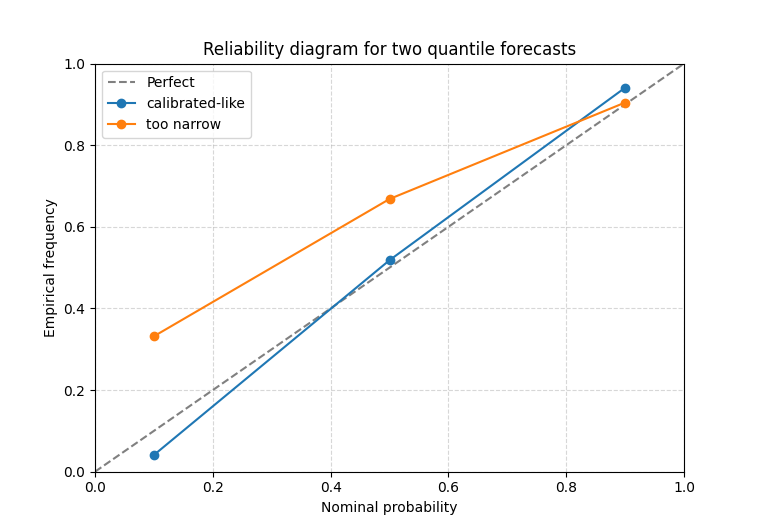
Read reliability for two quantile forecasts

In this mode the x-axis is the nominal quantile level itself:

• 0.10,

• 0.50,

• 0.90.

The y-axis is the observed proportion of cases where the true value falls below the corresponding predicted quantile.

A well-calibrated quantile forecast should therefore stay close to the diagonal. That is why this figure is so useful for teaching: it directly compares what the forecast claimed against what happened.

plot_reliability_diagram(
    {
        "calibrated-like": good_df,
        "too narrow": bad_df,
    },
    quantiles=quantiles,
    q_prefix="subsidence",
    actual_col="subsidence_actual",
    title="Reliability diagram for two quantile forecasts",
    figsize=(7.6, 5.3),
    grid_props={"linestyle": "--", "alpha": 0.5},
)

[INFO] Processing model 'calibrated-like'
[INFO] Processing model 'too narrow'

<Axes: title={'center': 'Reliability diagram for two quantile forecasts'}, xlabel='Nominal probability', ylabel='Empirical frequency'>

How to read the quantile case

A practical reading strategy is:

1. look at the highest quantile first,

2. then the lowest quantile,

3. then check whether the middle quantile is also drifting.

For example:

• if the point at q=0.90 lies well below 0.90, the upper band is too low or the forecast spread is too narrow,

• if the point at q=0.10 lies above 0.10, the lower quantile is not low enough,

• if the whole curve sits above or below the diagonal, that often reflects a systematic location bias.

In other words, the reliability diagram is not only a pass/fail plot. It tells you where the calibration problem is.

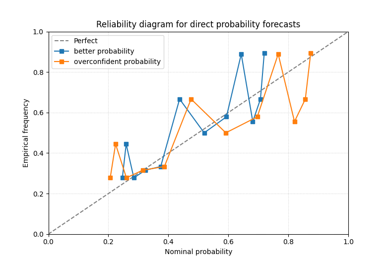
A direct-probability example

The same helper can also read direct probabilities.

Here the forecast is not a full quantile table. Instead, it predicts the probability of a binary event, for example:

• exceedance of a subsidence threshold,

• occurrence of a critical warning class,

• or any yes/no event of operational interest.

We create one better probability forecast and one overconfident one.

p_base = 1.0 / (1.0 + np.exp(-(np.sin(x / 2.5) + 0.2 * np.cos(x / 4.0))))
event_flag = rng.binomial(1, np.clip(p_base, 0.02, 0.98), size=n)

prob_df_good = pd.DataFrame(
    {
        "p_event": np.clip(0.92 * p_base + 0.03, 0.01, 0.99),
        "event_flag": event_flag,
    }
)

prob_df_bad = pd.DataFrame(
    {
        "p_event": np.clip(1.30 * p_base - 0.10, 0.01, 0.99),
        "event_flag": event_flag,
    }
)

print("\nDirect-probability preview")
print(
    pd.concat(
        {
            "better_prob": prob_df_good.head(6),
            "overconfident_prob": prob_df_bad.head(6),
        },
        axis=1,
    )
)

Direct-probability preview
  better_prob            overconfident_prob
      p_event event_flag            p_event event_flag
0      0.5358          1             0.6148          1
1      0.5424          1             0.6240          1
2      0.5488          0             0.6331          0
3      0.5553          1             0.6422          1
4      0.5616          1             0.6512          1
5      0.5679          1             0.6601          1

Use probability bins instead of quantile levels

In the probability mode, the helper bins the forecast probabilities.

With bin_strategy='uniform', the bins are evenly spaced in [0, 1]. With bin_strategy='quantile', the bins try to hold a similar number of samples.

The quantile strategy is often easier to read when the probabilities are concentrated in a narrow range.

plot_reliability_diagram(
    {
        "better probability": prob_df_good,
        "overconfident probability": prob_df_bad,
    },
    prob_col="p_event",
    actual_col="event_flag",
    bins=12,
    bin_strategy="quantile",
    title="Reliability diagram for direct probability forecasts",
    figsize=(7.8, 5.3),
    grid_props={"linestyle": ":", "alpha": 0.65},
)

[INFO] Processing model 'better probability'
[INFO] Processing model 'overconfident probability'

<Axes: title={'center': 'Reliability diagram for direct probability forecasts'}, xlabel='Nominal probability', ylabel='Empirical frequency'>

Why this bridge page is valuable

This page belongs naturally near uncertainty teaching because it connects saved forecast tables to calibration thinking without requiring the user to build arrays manually.

The function is especially useful when you want to answer:

• are my quantiles believable?

• are my exceedance probabilities trustworthy?

• did one model become overconfident?

• does a forecast that looks sharp actually misrepresent uncertainty?

It is therefore a strong bridge between forecast-table exploration and evaluation-minded reliability reading.

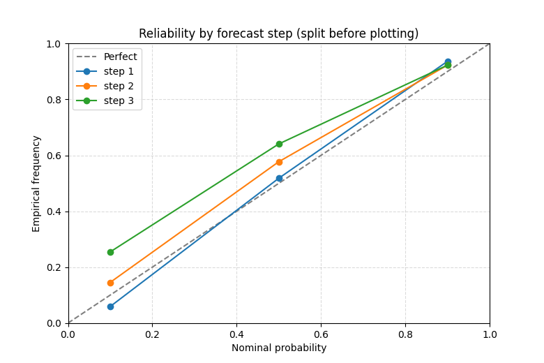
A grouped horizon example for forecast tables

Many forecast tables are long-format and contain a horizon or step column. The plotting helper itself does not draw one line per group, but the typical workflow is still very educational:

• filter one horizon at a time,

• or create a small dict of horizon-specific tables,

• then compare reliability across those subsets.

Here we build a quick long table and then split it into step-specific model labels to make the idea concrete.

step_frames = []
for step, bias, scale in [(1, 0.00, 0.75), (2, 0.10, 0.62), (3, 0.22, 0.50)]:
    center = center_good + bias
    spread = scale + 0.06 * np.sin(x / 4.0)
    frame = pd.DataFrame(
        {
            "forecast_step": step,
            "subsidence_q10": center + spread * z10,
            "subsidence_q50": center + spread * z50,
            "subsidence_q90": center + spread * z90,
            "subsidence_actual": y_true,
        }
    )
    step_frames.append(frame)

long_df = pd.concat(step_frames, ignore_index=True)

step_models = {
    f"step {step}": long_df[long_df["forecast_step"] == step].copy()
    for step in sorted(long_df["forecast_step"].unique())
}

plot_reliability_diagram(
    step_models,
    quantiles=quantiles,
    q_prefix="subsidence",
    actual_col="subsidence_actual",
    title="Reliability by forecast step (split before plotting)",
    figsize=(7.8, 5.2),
    grid_props={"linestyle": "--", "alpha": 0.45},
)

[INFO] Processing model 'step 1'
[INFO] Processing model 'step 2'
[INFO] Processing model 'step 3'

<Axes: title={'center': 'Reliability by forecast step (split before plotting)'}, xlabel='Nominal probability', ylabel='Empirical frequency'>

Practical checklist for your own data

When adapting this helper to a real project, a safe checklist is:

1. decide whether you are in the quantile or probability mode,

2. confirm the required columns exist,

3. start with one model or one horizon before comparing many curves,

4. prefer bin_strategy='quantile' when probabilities cluster,

5. interpret the diagonal together with interval sharpness or WIS.

For quantile tables:

• set q_prefix to the shared base name,

• pass the nominal levels as quantiles,

• and point actual_col to the observed target.

For probability tables:

• pass prob_col and a binary actual_col,

• choose a sensible number of bins,

• and check whether the empirical frequencies drift above or below the nominal probability scale.

This helper is often the fastest way to see whether uncertainty predictions are trustworthy enough to justify deeper calibration work or whether a model is already well behaved.