
Note
Go to the end to download the full example code.
Inspect physics-payload metadata before opening the full payload#
This lesson explains how to inspect a physics-payload metadata
sidecar, usually a file such as physics_payload.npz.meta.json.
This artifact is small, but it carries some of the most important semantic information attached to an exported physics payload:
which model and split produced the payload,
which PDE modes were active,
which groundwater convention was used,
which closure / tau-prior definition was assumed,
which units should be used when interpreting the arrays,
and which compact epsilon-style payload metrics were recorded.
The goal of this page is therefore not only to call helper functions. It is to teach how to inspect the metadata first, so a user can decide whether the heavier NPZ payload is worth opening and whether its conventions match the intended analysis.
from __future__ import annotations

import json
import tempfile
from pathlib import Path
from pprint import pprint

import matplotlib.pyplot as plt
import pandas as pd

from geoprior.utils.inspect import (
    generate_physics_payload_meta,
    inspect_physics_payload_meta,
    load_physics_payload_meta,
    physics_payload_meta_closure_frame,
    physics_payload_meta_identity_frame,
    physics_payload_meta_metrics_frame,
    physics_payload_meta_units_frame,
    plot_physics_payload_meta_boolean_summary,
    plot_physics_payload_meta_core_scalars,
    plot_physics_payload_meta_payload_metrics,
    summarize_physics_payload_meta,
)

pd.set_option("display.max_columns", 30)
pd.set_option("display.width", 112)
pd.set_option("display.max_colwidth", 88)


PAYLOAD_META_PALETTE = {
    "core": "#0F766E",
    "metrics": "#7C3AED",
    "pass": "#15803D",
    "fail": "#B91C1C",
    "edge": "#334155",
    "panel": "#FCFCFE",
}


def _style_bar_panel(
    ax: plt.Axes,
    *,
    color: str,
    edge: str = PAYLOAD_META_PALETTE["edge"],
) -> None:
    """Polish a bar-based gallery panel."""
    for patch in ax.patches:
        patch.set_facecolor(color)
        patch.set_edgecolor(edge)
        patch.set_linewidth(1.25)
        patch.set_alpha(0.94)
    ax.set_facecolor(PAYLOAD_META_PALETTE["panel"])
    ax.tick_params(labelsize=9)
    ax.title.set_fontweight("bold")
    for side in ("top", "right"):
        ax.spines[side].set_visible(False)
    for side in ("left", "bottom"):
        ax.spines[side].set_color("#CBD5E1")


def _style_boolean_panel(ax: plt.Axes) -> None:
    """Apply a distinct pass/fail palette to boolean panels."""
    for patch in ax.patches:
        width = patch.get_width()
        height = patch.get_height()
        score = width if width != 0 else height
        color = (
            PAYLOAD_META_PALETTE["pass"]
            if score >= 0.5
            else PAYLOAD_META_PALETTE["fail"]
        )
        patch.set_facecolor(color)
        patch.set_edgecolor(PAYLOAD_META_PALETTE["edge"])
        patch.set_linewidth(1.15)
        patch.set_alpha(0.94)
    ax.set_facecolor(PAYLOAD_META_PALETTE["panel"])
    ax.tick_params(labelsize=9)
    ax.title.set_fontweight("bold")
    for side in ("top", "right"):
        ax.spines[side].set_visible(False)
    for side in ("left", "bottom"):
        ax.spines[side].set_color("#CBD5E1")
Why this artifact matters#
The full physics payload is often an NPZ archive that stores heavy arrays. Opening it directly can be unnecessary if the exported run already uses conventions or closures that do not match the question we want to study.
The metadata sidecar is therefore the ideal first checkpoint. It lets us answer practical questions such as:
Was this payload produced by the model and split I expected?
Were both
consolidationandgw_flowactive, or only one?Are groundwater values interpreted as depth below ground or something else?
Which tau-prior / closure formula was used to define the saved residual context?
Are the saved units compatible with the way I plan to report results or compare payloads across runs?
In other words, this artifact is a semantic filter. It helps the user validate meaning before reading arrays.
Create a realistic demo metadata sidecar#
For documentation pages, we want a stable artifact that behaves like a real metadata sidecar without rebuilding a full physics payload. The generation helper was designed exactly for that use case.
Here we create a metadata file with realistic identity fields, unit conventions, closure definitions, and compact payload metrics.
out_dir = Path(tempfile.mkdtemp(prefix="gp_payload_meta_"))
meta_path = out_dir / "physics_payload_demo.npz.meta.json"

generate_physics_payload_meta(
    meta_path,
    city="nansha",
    model_name="GeoPriorSubsNet",
    split="TestSet",
    created_utc="2026-03-30T10:18:55Z",
    pde_modes_active=["consolidation", "gw_flow"],
    time_units="year",
    time_coord_units="year",
    gwl_kind="depth_bgs",
    gwl_sign="down_positive",
    use_head_proxy=True,
    kappa_mode="kb",
    use_effective_h=True,
    hd_factor=0.6,
    lambda_offset=1.0,
    kappa_value=0.04639,
    tau_prior_definition="tau_closure_from_learned_fields",
    tau_prior_human_name="tau_closure",
    tau_prior_source="model.evaluate_physics() closure head",
    tau_closure_formula="Hd^2 * Ss / (pi^2 * kappa_b * K)",
    payload_metrics={
        "eps_prior_rms": 3.57e-4,
        "eps_cons_scaled_rms": 2.61e-6,
        "closure_consistency_rms": None,
        "r2_logtau": 1.0,
        "kappa_used_for_closure": None,
    },
)

print("Written physics-payload metadata file")
print(f" - {meta_path}")
Written physics-payload metadata file
 - /tmp/gp_payload_meta_n8_xcj09/physics_payload_demo.npz.meta.json
Load the artifact with the real reader#
Even in a lesson, it is worth using the same loading entry point a real workflow would use. That keeps the page close to a user’s actual inspection path.
meta_record = load_physics_payload_meta(meta_path)

print("\nArtifact header")
pprint(
    {
        "kind": meta_record.kind,
        "stage": meta_record.stage,
        "city": meta_record.city,
        "model": meta_record.model,
        "path": str(meta_record.path),
    }
)
Artifact header
{'city': 'nansha',
 'kind': 'physics_payload_meta',
 'model': 'GeoPriorSubsNet',
 'path': '/tmp/gp_payload_meta_n8_xcj09/physics_payload_demo.npz.meta.json',
 'stage': None}
Start with the compact semantic summary#
Before opening every table, start with the compact summary.
This summary is useful because it reorganizes the raw metadata into a few inspection layers:
a short identity block,
conventions for groundwater and time,
closure / tau-prior semantics,
payload-level metrics,
and boolean checks for structural completeness.
When you inspect many payload exports, this summary is often the fastest way to reject a mismatched sidecar before reading more.
summary = summarize_physics_payload_meta(meta_record)

print("\nCompact summary")
print(json.dumps(summary, indent=2))
Compact summary
{
  "brief": {
    "kind": "physics_payload_meta",
    "created_utc": "2026-03-30T10:18:55Z",
    "saved_utc": "2026-03-30T10:18:55Z",
    "model_name": "GeoPriorSubsNet",
    "city": "nansha",
    "split": "TestSet",
    "pde_modes_active": [
      "consolidation",
      "gw_flow"
    ],
    "n_pde_modes": 2
  },
  "conventions": {
    "time_units": "year",
    "time_coord_units": "year",
    "gwl_kind": "depth_bgs",
    "gwl_sign": "down_positive",
    "use_head_proxy": true,
    "kappa_mode": "kb"
  },
  "closure": {
    "tau_prior_definition": "tau_closure_from_learned_fields",
    "tau_prior_human_name": "tau_closure",
    "tau_prior_source": "model.evaluate_physics() closure head",
    "tau_closure_formula": "Hd^2 * Ss / (pi^2 * kappa_b * K)",
    "use_effective_h": true,
    "use_effective_thickness": true,
    "hd_factor": 0.6,
    "Hd_factor": 0.6,
    "kappa_value": 0.04639
  },
  "payload_metrics": {
    "eps_prior_rms": 0.000357,
    "eps_cons_scaled_rms": 2.61e-06,
    "r2_logtau": 1.0
  },
  "units": {
    "n_units": 8,
    "quantities": [
      "H",
      "Hd",
      "K",
      "Ss",
      "cons_res_vals",
      "kappa",
      "tau",
      "tau_prior"
    ],
    "tau_unit": "s",
    "tau_prior_unit": "s",
    "K_unit": "m/s",
    "Ss_unit": "1/m"
  },
  "checks": {
    "has_model_name": true,
    "has_city": true,
    "has_split": true,
    "has_pde_modes": true,
    "has_units": true,
    "has_payload_metrics": true,
    "has_tau_prior_definition": true,
    "has_tau_closure_formula": true,
    "time_units_present": true,
    "time_coord_units_present": true,
    "kappa_value_present": true,
    "lambda_offset_present": true,
    "hd_factor_present": true,
    "payload_eps_prior_present": true,
    "payload_eps_cons_present": true,
    "uses_head_proxy": true
  },
  "core_scalars": {
    "hd_factor": 0.6,
    "lambda_offset": 1.0,
    "Hd_factor": 0.6,
    "lambda_offsets": 1.0,
    "kappa_value": 0.04639
  }
}
Read the identity frame first#
The identity frame answers the first practical question:
What exactly does this metadata sidecar describe?
This is where we verify model name, city, split, PDE modes, time units, and groundwater conventions.
In practice, this frame is often the quickest way to catch mistakes such as:
opening a payload from the wrong split,
mixing runs built with different PDE modes,
or confusing groundwater depth conventions.
Identity and convention view
               field                   value
0        created_utc    2026-03-30T10:18:55Z
1          saved_utc    2026-03-30T10:18:55Z
2         model_name         GeoPriorSubsNet
3               city                  nansha
4              split                 TestSet
5         time_units                    year
6   time_coord_units                    year
7           gwl_kind               depth_bgs
8           gwl_sign           down_positive
9     use_head_proxy                    True
10        kappa_mode                      kb
11  pde_modes_active  consolidation, gw_flow
Read the closure frame carefully#
The closure frame is one of the most important parts of this artifact family.
It tells us how the payload relates its physical fields to the tau prior and whether effective thickness was used. This matters because two payloads can look similar numerically while encoding different closure assumptions.
When this frame changes across experiments, the comparison is not purely a metric comparison anymore. It becomes a modeling-choice comparison.
Closure / tau-prior view
                     field                                  value
0     tau_prior_definition        tau_closure_from_learned_fields
1     tau_prior_human_name                            tau_closure
2         tau_prior_source  model.evaluate_physics() closure head
3      tau_closure_formula       Hd^2 * Ss / (pi^2 * kappa_b * K)
4          use_effective_h                                   True
5  use_effective_thickness                                   True
6                hd_factor                               0.600000
7                Hd_factor                               0.600000
8              kappa_value                               0.046390
Inspect the units before opening arrays#
The units block is the safeguard that prevents misreading the NPZ
payload. A user should not interpret fields such as K, Ss,
tau, or residual values before checking the declared units.
A healthy reading pattern is:
verify that the expected physical quantities are present,
check that
tauandtau_priorshare compatible units,confirm that the residual values are expressed in the units you expect for later reporting.
Units block
        quantity           unit
0              H              m
1             Hd              m
2              K            m/s
3             Ss            1/m
4  cons_res_vals            m/s
5          kappa  dimensionless
6            tau              s
7      tau_prior              s
Read the compact payload metrics#
The payload metrics are not a replacement for the full evaluation artifact. They are a compact checkpoint attached directly to the exported payload.
In this lesson, the most informative metrics are usually:
eps_prior_rmseps_cons_scaled_rmsclosure_consistency_rmsr2_logtaukappa_used_for_closure
Together they help answer a small but important question:
Does this payload still carry a physically interpretable closure context, or does it already look inconsistent before I read the heavier arrays?
Payload metrics
           section               metric    value
0  payload_metrics  eps_cons_scaled_rms 0.000003
1  payload_metrics        eps_prior_rms 0.000357
2  payload_metrics            r2_logtau 1.000000
Use the all-in-one inspector when you want the key tables together#
inspect_physics_payload_meta(...) is useful when you want a
compact bundle with:
the semantic summary,
the identity frame,
the closure frame,
the units frame,
and the metrics frame.
This is especially useful for batch inspection tools that need to scan many sidecars quickly before deciding which payload archives deserve a deeper review.
Inspector bundle keys
['closure_frame', 'identity_frame', 'metrics_frame', 'summary', 'units_frame']
Plot the metadata scalars and payload metrics#
The first figure answers two different questions.
The core scalars plot shows top-level numeric metadata such as
hd_factor, Hd_factor, lambda_offset, and kappa_value.
This helps the user check whether the saved payload corresponds to the physical closure settings they intended.
The payload metrics plot then summarizes the small diagnostic numbers attached directly to the payload. This is a quick way to see whether epsilon-like values are tiny, moderate, or obviously suspicious.
fig, axes = plt.subplots(
    1,
    2,
    figsize=(12.4, 4.8),
    constrained_layout=True,
)

plot_physics_payload_meta_core_scalars(
    meta_record,
    ax=axes[0],
    title="Physics-payload meta: core scalars",
)
_style_bar_panel(axes[0], color=PAYLOAD_META_PALETTE["core"])
plot_physics_payload_meta_payload_metrics(
    meta_record,
    ax=axes[1],
    title="Physics-payload meta: payload metrics",
)
_style_bar_panel(axes[1], color=PAYLOAD_META_PALETTE["metrics"], edge="#4C1D95")
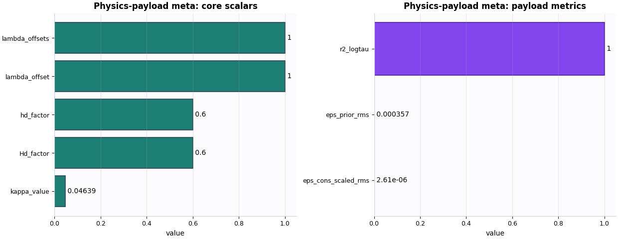
How should you read these two plots?#
A good reading strategy is:
use the left plot to confirm that the saved metadata still reflects the closure regime you intended,
use the right plot to judge whether the payload-level epsilon values remain small enough to support a later deeper read.
Not every project will use the same thresholds, but some common warning signs are:
missing or null critical scalars,
unexpectedly different
hd_factororkappa_valuebetween runs you thought were comparable,very large epsilon-style metrics compared with your usual runs,
or missing payload metrics when you expected the exporter to attach them.
Plot the structural decision checks separately#
The boolean summary is useful because it turns the metadata into a compact pass/fail-style review:
identity present,
PDE modes present,
units present,
closure definition present,
payload metrics present,
key physical scalars present.
This is the fastest plot for deciding whether a sidecar is ready for serious downstream inspection.
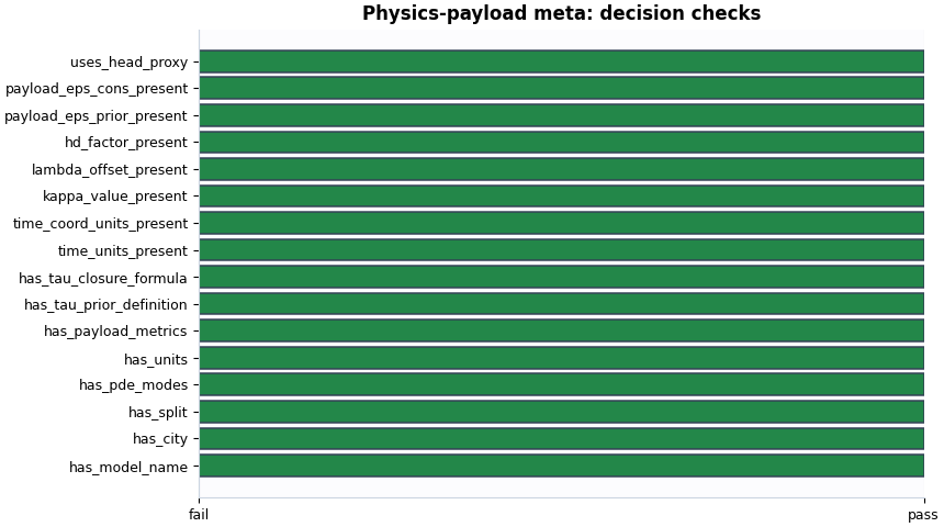
A practical reading rule#
For this artifact family, a useful first-pass decision rule can be:
model, city, and split are present,
PDE modes are recorded,
units are present,
tau-prior definition and closure formula are present,
payload metrics are present,
and the key scalar fields such as
kappa_valueandlambda_offsetare not missing.
If these checks pass, the metadata is usually healthy enough for the user to open the heavier NPZ payload with confidence.
checks = summary["checks"]
must_pass = [
    "has_model_name",
    "has_city",
    "has_split",
    "has_pde_modes",
    "has_units",
    "has_payload_metrics",
    "has_tau_prior_definition",
    "has_tau_closure_formula",
    "time_units_present",
    "time_coord_units_present",
    "kappa_value_present",
    "lambda_offset_present",
    "hd_factor_present",
]
ready = all(bool(checks.get(name, False)) for name in must_pass)

print("\nDecision note")
if ready:
    print(
        "This metadata sidecar looks structurally ready for a "
        "deeper read of the full physics payload archive."
    )
else:
    print(
        "This metadata sidecar needs attention before you rely "
        "on the heavier payload it describes."
    )
Decision note
This metadata sidecar looks structurally ready for a deeper read of the full physics payload archive.
Total running time of the script: (0 minutes 0.348 seconds)