
Note
Go to the end to download the full example code.
Extend forecast CSVs to later years#
This example teaches you how to use GeoPrior’s
extend-forecast utility.
Unlike the plotting scripts, this command is a forecast-product builder. It takes an existing future forecast CSV and extends it to one or more later years by simple extrapolation.
Why this matters#
In many workflows, the trained model only emits forecasts to a fixed horizon, but downstream reporting still needs:
one or two extra years,
a quick scenario extension,
or a compact artifact for later mapping and hotspot analysis.
This builder helps create those extended future CSVs directly from existing forecast exports.
Imports#
We call the real production entrypoint from the project code. Then we read the generated CSVs back in and build one compact teaching preview.
from __future__ import annotations

import tempfile
from pathlib import Path

import matplotlib.pyplot as plt
import numpy as np
import pandas as pd

from geoprior.scripts.extend_forecast import (
    extend_forecast_main,
)
Build compact synthetic forecast archives#
The production builder resolves, per city:
one eval CSV,
one future CSV,
and then extends the future horizon.
For the lesson, we create synthetic cumulative forecast archives for:
Nansha
Zhongshan
with:
eval years = 2020, 2021, 2022
future years = 2023, 2024, 2025
The synthetic paths are designed so that:
Zhongshan has a higher cumulative level,
the final years contain a clean trend,
and uncertainty widens gently with horizon.
rng = np.random.default_rng(21)

eval_years = [2020, 2021, 2022]
future_years = [2023, 2024, 2025]
n_points = 70


def _city_forecasts(
    *,
    city: str,
    base_shift: float,
    trend_shift: float,
) -> tuple[pd.DataFrame, pd.DataFrame]:
    rows_eval: list[dict[str, object]] = []
    rows_future: list[dict[str, object]] = []

    for sample_idx in range(n_points):
        x = 100.0 + 0.55 * sample_idx
        y = 250.0 + 0.18 * sample_idx

        local = rng.normal(0.0, 1.2)
        slope = 14.0 + trend_shift + 0.03 * sample_idx + local
        start = 18.0 + base_shift + 0.35 * sample_idx

        # Annual increments.
        inc_2020 = start
        inc_2021 = start + 0.65 * slope
        inc_2022 = start + 1.00 * slope
        inc_2023 = start + 1.28 * slope
        inc_2024 = start + 1.55 * slope
        inc_2025 = start + 1.83 * slope

        # Cumulative q50 path.
        q50_2020 = inc_2020
        q50_2021 = q50_2020 + inc_2021
        q50_2022 = q50_2021 + inc_2022
        q50_2023 = q50_2022 + inc_2023
        q50_2024 = q50_2023 + inc_2024
        q50_2025 = q50_2024 + inc_2025

        # Eval actuals.
        act_2020 = max(0.1, q50_2020 + rng.normal(0.0, 2.0))
        act_2021 = max(0.1, q50_2021 + rng.normal(0.0, 2.5))
        act_2022 = max(0.1, q50_2022 + rng.normal(0.0, 3.0))

        def _band(center: float, year: int) -> tuple[float, float]:
            width = 8.0 + 0.7 * (year - 2020)
            return max(0.0, center - width), center + width

        for step, (year, q50, actual) in enumerate(
            [
                (2020, q50_2020, act_2020),
                (2021, q50_2021, act_2021),
                (2022, q50_2022, act_2022),
            ],
            start=1,
        ):

            q10, q90 = _band(q50, year)
            rows_eval.append(
                {
                    "city": city,
                    "sample_idx": sample_idx,
                    "forecast_step": step,
                    "coord_x": float(x),
                    "coord_y": float(y),
                    "coord_t": int(year),
                    "subsidence_actual": float(actual),
                    "subsidence_q10": float(q10),
                    "subsidence_q50": float(q50),
                    "subsidence_q90": float(q90),
                    "subsidence_unit": "mm",
                }
            )

        # Future rows
        for step, (year, q50) in enumerate(
            [
                (2023, q50_2023),
                (2024, q50_2024),
                (2025, q50_2025),
            ],
            start=1,
        ):
            q10, q90 = _band(q50, year)
            rows_future.append(
                {
                    "city": city,
                    "sample_idx": sample_idx,
                    "forecast_step": step,
                    "coord_x": float(x),
                    "coord_y": float(y),
                    "coord_t": int(year),
                    "subsidence_q10": float(q10),
                    "subsidence_q50": float(q50),
                    "subsidence_q90": float(q90),
                    "subsidence_unit": "mm",
                }
            )

    return pd.DataFrame(rows_eval), pd.DataFrame(rows_future)


ns_eval_df, ns_future_df = _city_forecasts(
    city="Nansha",
    base_shift=0.0,
    trend_shift=0.0,
)
zh_eval_df, zh_future_df = _city_forecasts(
    city="Zhongshan",
    base_shift=8.0,
    trend_shift=1.8,
)

print("Nansha future preview")
print(ns_future_df.head(6).to_string(index=False))

print("")
print("Zhongshan future preview")
print(zh_future_df.head(6).to_string(index=False))
Nansha future preview
  city  sample_idx  forecast_step  coord_x  coord_y  coord_t  subsidence_q10  subsidence_q50  subsidence_q90 subsidence_unit
Nansha           0              1 100.0000 250.0000     2023        104.1814        114.2814        124.3814              mm
Nansha           0              2 100.0000 250.0000     2024        143.8488        154.6488        165.4488              mm
Nansha           0              3 100.0000 250.0000     2025        187.5566        199.0566        210.5566              mm
Nansha           1              1 100.5500 250.1800     2023        104.2415        114.3415        124.4415              mm
Nansha           1              2 100.5500 250.1800     2024        143.5500        154.3500        165.1500              mm
Nansha           1              3 100.5500 250.1800     2025        186.7710        198.2710        209.7710              mm

Zhongshan future preview
     city  sample_idx  forecast_step  coord_x  coord_y  coord_t  subsidence_q10  subsidence_q50  subsidence_q90 subsidence_unit
Zhongshan           0              1 100.0000 250.0000     2023        136.6795        146.7795        156.8795              mm
Zhongshan           0              2 100.0000 250.0000     2024        184.6103        195.4103        206.2103              mm
Zhongshan           0              3 100.0000 250.0000     2025        236.6292        248.1292        259.6292              mm
Zhongshan           1              1 100.5500 250.1800     2023        145.4446        155.5446        165.6446              mm
Zhongshan           1              2 100.5500 250.1800     2024        197.6216        208.4216        219.2216              mm
Zhongshan           1              3 100.5500 250.1800     2025        254.5905        266.0905        277.5905              mm
Write the synthetic CSV inputs#
The production command works from CSV files, so the lesson keeps the same workflow.
tmp_dir = Path(
    tempfile.mkdtemp(prefix="gp_sg_extend_forecast_")
)

ns_eval_csv = tmp_dir / "nansha_eval.csv"
ns_future_csv = tmp_dir / "nansha_future.csv"
zh_eval_csv = tmp_dir / "zhongshan_eval.csv"
zh_future_csv = tmp_dir / "zhongshan_future.csv"

ns_eval_df.to_csv(ns_eval_csv, index=False)
ns_future_df.to_csv(ns_future_csv, index=False)
zh_eval_df.to_csv(zh_eval_csv, index=False)
zh_future_df.to_csv(zh_future_csv, index=False)

print("")
print("Input files")
for p in [
    ns_eval_csv,
    ns_future_csv,
    zh_eval_csv,
    zh_future_csv,
]:
    print(" -", p.name)
Input files
 - nansha_eval.csv
 - nansha_future.csv
 - zhongshan_eval.csv
 - zhongshan_future.csv
Run the real forecast-extension builder#
We ask the builder to:
interpret the inputs as cumulative subsidence,
keep the output in cumulative form,
extend to the explicit years 2026 and 2027,
use a short linear-fit window,
and widen uncertainty with a sqrt rule.
Because we request both cities, the script writes one CSV per city with a city suffix added to the output stem.
out_stem = tmp_dir / "future_extended_gallery.csv"

extend_forecast_main(
    [
        "--ns-eval",
        str(ns_eval_csv),
        "--ns-future",
        str(ns_future_csv),
        "--zh-eval",
        str(zh_eval_csv),
        "--zh-future",
        str(zh_future_csv),
        "--subsidence-kind",
        "cumulative",
        "--out-kind",
        "same",
        "--method",
        "linear_fit",
        "--window",
        "3",
        "--years",
        "2026",
        "2027",
        "--unc-growth",
        "sqrt",
        "--unc-scale",
        "1.0",
        "--out",
        str(out_stem),
    ],
    prog="extend-forecast",
)
[OK] Nansha: wrote /tmp/gp_sg_extend_forecast_y2mw5jor/future_extended_gallery_nansha.csv (manual)
[OK] Zhongshan: wrote /tmp/gp_sg_extend_forecast_y2mw5jor/future_extended_gallery_zhongshan.csv (manual)
Inspect the produced files#
The builder writes one output CSV per city in multi-city mode.
Written files
 - future_extended_gallery_nansha.csv
 - future_extended_gallery_zhongshan.csv
Read the extended outputs#
We read both city-level outputs back in and inspect the newly added years.
def _pick_city_output(paths: list[Path], city_slug: str) -> Path:
    for p in paths:
        if city_slug in p.name.lower():
            return p
    raise FileNotFoundError(city_slug)


ns_out_csv = _pick_city_output(written, "nansha")
zh_out_csv = _pick_city_output(written, "zhongshan")

ns_ext = pd.read_csv(ns_out_csv)
zh_ext = pd.read_csv(zh_out_csv)

print("")
print("Extended Nansha output")
print(
    ns_ext.loc[ns_ext["coord_t"].isin([2025, 2026, 2027])]
    .head(8)
    .to_string(index=False)
)

print("")
print("Extended Zhongshan output")
print(
    zh_ext.loc[zh_ext["coord_t"].isin([2025, 2026, 2027])]
    .head(8)
    .to_string(index=False)
)
Extended Nansha output
  city  sample_idx  forecast_step  coord_x  coord_y  coord_t  subsidence_q10  subsidence_q50  subsidence_q90 subsidence_unit extended extend_kind extend_method unc_growth
Nansha           0              3 100.0000 250.0000     2025        187.5566        199.0566        210.5566              mm      NaN         NaN           NaN        NaN
   NaN           0              4 100.0000 250.0000     2026        234.9189        247.4088        259.8988              mm     True  cumulative    linear_fit       sqrt
   NaN           0              5 100.0000 250.0000     2027        286.0671        299.7695        313.4719              mm     True  cumulative    linear_fit       sqrt
Nansha           1              3 100.5500 250.1800     2025        186.7710        198.2710        209.7710              mm      NaN         NaN           NaN        NaN
   NaN           1              4 100.5500 250.1800     2026        233.5214        246.0114        258.5013              mm     True  cumulative    linear_fit       sqrt
   NaN           1              5 100.5500 250.1800     2027        283.9308        297.6331        311.3355              mm     True  cumulative    linear_fit       sqrt
Nansha           2              3 101.1000 250.3600     2025        187.7252        199.2252        210.7252              mm      NaN         NaN           NaN        NaN
   NaN           2              4 101.1000 250.3600     2026        234.4436        246.9335        259.4235              mm     True  cumulative    linear_fit       sqrt

Extended Zhongshan output
     city  sample_idx  forecast_step  coord_x  coord_y  coord_t  subsidence_q10  subsidence_q50  subsidence_q90 subsidence_unit extended extend_kind extend_method unc_growth
Zhongshan           0              3 100.0000 250.0000     2025        236.6292        248.1292        259.6292              mm      NaN         NaN           NaN        NaN
      NaN           0              4 100.0000 250.0000     2026        292.3490        304.8389        317.3289              mm     True  cumulative    linear_fit       sqrt
      NaN           0              5 100.0000 250.0000     2027        351.9020        365.6044        379.3068              mm     True  cumulative    linear_fit       sqrt
Zhongshan           1              3 100.5500 250.1800     2025        254.5905        266.0905        277.5905              mm      NaN         NaN           NaN        NaN
      NaN           1              4 100.5500 250.1800     2026        315.9474        328.4374        340.9273              mm     True  cumulative    linear_fit       sqrt
      NaN           1              5 100.5500 250.1800     2027        381.8358        395.5382        409.2405              mm     True  cumulative    linear_fit       sqrt
Zhongshan           2              3 101.1000 250.3600     2025        247.6953        259.1953        270.6953              mm      NaN         NaN           NaN        NaN
      NaN           2              4 101.1000 250.3600     2026        306.4038        318.8937        331.3837              mm     True  cumulative    linear_fit       sqrt
Summarize before vs after#
A compact summary makes the extension behavior clearer.
We compute city-level mean q10/q50/q90 paths before and after the extension.
def _mean_path(df: pd.DataFrame) -> pd.DataFrame:
    return (
        df.groupby("coord_t", as_index=False)[
            ["subsidence_q10", "subsidence_q50", "subsidence_q90"]
        ]
        .mean()
        .sort_values("coord_t")
    )


ns_before = _mean_path(ns_future_df)
zh_before = _mean_path(zh_future_df)
ns_after = _mean_path(ns_ext)
zh_after = _mean_path(zh_ext)

print("")
print("Mean Nansha path after extension")
print(ns_after.to_string(index=False))

print("")
print("Mean Zhongshan path after extension")
print(zh_after.to_string(index=False))
Mean Nansha path after extension
 coord_t  subsidence_q10  subsidence_q50  subsidence_q90
    2023        154.1724        164.2724        174.3724
    2024        206.8092        217.6092        228.4092
    2025        263.6481        275.1481        286.6481
    2026        324.2992        336.7892        349.2791
    2027        388.8966        402.5990        416.3014

Mean Zhongshan path after extension
 coord_t  subsidence_q10  subsidence_q50  subsidence_q90
    2023        192.5489        202.6489        212.7489
    2024        256.5590        267.3590        278.1590
    2025        325.3806        336.8806        348.3806
    2026        398.6091        411.0991        423.5890
    2027        476.3885        490.0909        503.7933
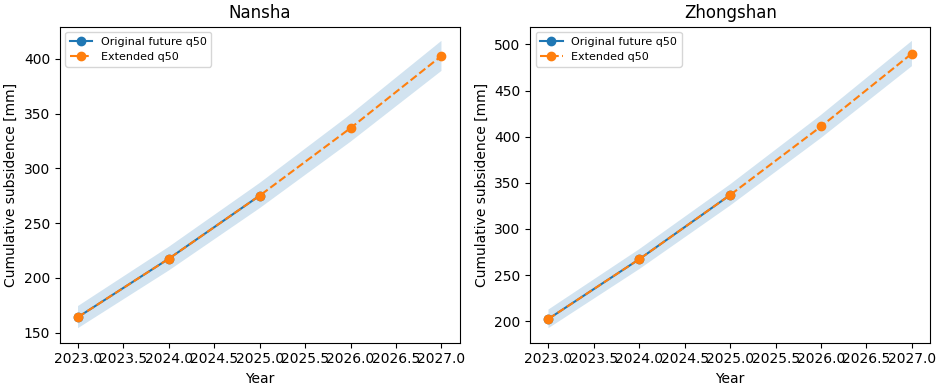
Build one compact visual preview#
This preview is not part of the production builder itself. It is a teaching aid for the gallery page.
- Left:
Nansha before/after q50 path.
- Right:
Zhongshan before/after q50 path.
The shaded ribbons show the q10-q90 interval after extension.
fig, axes = plt.subplots(
    1,
    2,
    figsize=(9.4, 3.9),
    constrained_layout=True,
)

for ax, city, before, after in [
    (axes[0], "Nansha", ns_before, ns_after),
    (axes[1], "Zhongshan", zh_before, zh_after),
]:
    ax.plot(
        before["coord_t"].to_numpy(int),
        before["subsidence_q50"].to_numpy(float),
        marker="o",
        label="Original future q50",
    )
    ax.plot(
        after["coord_t"].to_numpy(int),
        after["subsidence_q50"].to_numpy(float),
        marker="o",
        linestyle="--",
        label="Extended q50",
    )
    ax.fill_between(
        after["coord_t"].to_numpy(int),
        after["subsidence_q10"].to_numpy(float),
        after["subsidence_q90"].to_numpy(float),
        alpha=0.2,
    )
    ax.set_title(city)
    ax.set_xlabel("Year")
    ax.set_ylabel("Cumulative subsidence [mm]")
    ax.legend(fontsize=8)
Learn how to read this builder#
The extension logic starts from an existing future forecast CSV. It does not retrain the model.
The practical reading order is:
inspect the original future path up to its last available year;
check which extension rule was requested;
verify the new years added to the tail;
inspect how the q10-q90 interval widens after extension.
In other words:
this is a forecast-product builder,
not a new model inference stage.
Explicit years vs add-years#
The script supports two extension styles.
- Explicit years:
add the exact years requested by
--years.- Add N years:
if
--yearsis omitted, append the next--add-yearsyears after the existing tail.
The lesson uses explicit years because it makes the page easier to read, but both workflows are supported by the real command.
Why subsidence-kind and out-kind matter#
The command distinguishes:
the meaning of the input series,
and the meaning of the output series.
subsidence-kindtells the builder whether the source CSV represents cumulative values or annual/rate-style values.
out-kindcontrols whether the written extension should stay in the same convention, or be converted to cumulative or rate form.
This is useful because later scripts may consume different forecast conventions.
Why uncertainty growth matters#
The extrapolated years are less certain than the original trained horizon, so the command exposes:
holdsqrtlinear
uncertainty-growth modes, plus an unc-scale multiplier.
The visual preview above makes that visible through the widening q10-q90 ribbon in 2026 and 2027.
Why this page belongs in tables_and_summaries#
This script produces a reusable forecast CSV artifact that later builders can consume.
A useful workflow is:
generate the original future forecast,
extend the future CSV if later years are needed,
pass the extended CSV to hotspot or spatial-summary builders,
only then move to paper-ready maps or narrative tables.
That keeps:
model inference,
forecast extrapolation,
and final visualization
clearly separated.
Command-line version#
The same lesson can be reproduced from the CLI.
Legacy dispatcher:
python -m scripts extend-forecast \
  --ns-eval results/nansha_eval.csv \
  --ns-future results/nansha_future.csv \
  --zh-eval results/zhongshan_eval.csv \
  --zh-future results/zhongshan_future.csv \
  --subsidence-kind cumulative \
  --out-kind same \
  --method linear_fit \
  --window 3 \
  --years 2026 2027 \
  --unc-growth sqrt \
  --out future_extended
Add the next 2 years instead:
python -m scripts extend-forecast \
  --ns-src results/nansha_run \
  --zh-src results/zhongshan_run \
  --split auto \
  --add-years 2 \
  --method linear_last \
  --out future_extended
Modern CLI:
geoprior build extend-forecast \
  --ns-src results/nansha_run \
  --zh-src results/zhongshan_run \
  --split auto \
  --add-years 2 \
  --subsidence-kind cumulative \
  --out-kind same \
  --method linear_fit \
  --window 3 \
  --unc-growth sqrt \
  --out future_extended
The gallery page teaches the builder. The command line reproduces it in a workflow.
Total running time of the script: (0 minutes 0.378 seconds)