
Note
Go to the end to download the full example code.
Group-validity masks for Stage-1 diagnostics#
This lesson teaches how to use the Stage-1 group-mask helpers in GeoPrior:
Why this page matters#
Before training begins, GeoPrior needs to know which spatial groups contain enough temporal coverage to support:
supervised training windows, and
forecast-time processing windows.
That logic is not hidden. It is exposed explicitly through the group-mask helpers.
What the real utilities do#
compute_group_masks builds two sets of valid groups:
valid_for_train: groups containing all required years in the lasttime_steps + horizonwindow;valid_for_forecast: groups containing all required years in the lasttime_stepswindow.
The returned GroupMasks object also exposes:
required_train_yearsrequired_forecast_yearskeep_for_processing: the union of the train-valid and forecast-valid groups.
Once those groups are known, filter_df_by_groups keeps only the
rows whose group identifiers appear in the chosen group table.
What this lesson teaches#
We will:
build a compact spatial-temporal dataset,
remove years from selected groups,
compute train-valid and forecast-valid masks,
inspect the returned
GroupMasksobject,filter the original DataFrame,
plot the resulting group status map.
This page is synthetic so it remains fully executable during the documentation build.
Imports#
import numpy as np
import pandas as pd
import matplotlib.pyplot as plt

from geoprior.utils.holdout_utils import (
    compute_group_masks,
    filter_df_by_groups,
)
Step 1 - Build a compact spatial-temporal dataset#
Each spatial location acts as one group observed over multiple years.
rng = np.random.default_rng(11)

nx = 8
ny = 6
years = list(range(2018, 2025))

xv = np.linspace(0.0, 12_000.0, nx)
yv = np.linspace(0.0, 8_000.0, ny)
X, Y = np.meshgrid(xv, yv)

x_flat = X.ravel()
y_flat = Y.ravel()

xn = (x_flat - x_flat.min()) / (x_flat.max() - x_flat.min())
yn = (y_flat - y_flat.min()) / (y_flat.max() - y_flat.min())

hotspot = np.exp(
    -(
        ((xn - 0.72) ** 2) / 0.020
        + ((yn - 0.34) ** 2) / 0.032
    )
)
gradient = 0.42 * xn + 0.22 * (1.0 - yn)

rows: list[dict[str, float | int]] = []

for gid in range(x_flat.size):
    base = 2.0 + 1.5 * gradient[gid] + 1.8 * hotspot[gid]

    for year in years:
        rows.append(
            {
                "group_id": gid,
                "coord_x": float(x_flat[gid]),
                "coord_y": float(y_flat[gid]),
                "year": int(year),
                "subsidence": float(
                    base
                    + 0.32 * (year - years[0])
                    + rng.normal(0.0, 0.08)
                ),
            }
        )

df = pd.DataFrame(rows)

print("Initial dataset shape:", df.shape)
print("")
print(df.head(10).to_string(index=False))
Initial dataset shape: (336, 5)

 group_id     coord_x  coord_y  year  subsidence
        0    0.000000      0.0  2018    2.332735
        0    0.000000      0.0  2019    2.758780
        0    0.000000      0.0  2020    3.067978
        0    0.000000      0.0  2021    3.249175
        0    0.000000      0.0  2022    3.586162
        0    0.000000      0.0  2023    3.887809
        0    0.000000      0.0  2024    4.295578
        1 1714.285714      0.0  2018    2.415515
        1 1714.285714      0.0  2019    2.799751
        1 1714.285714      0.0  2020    2.912214
Step 2 - Remove years from selected groups#
We deliberately create three kinds of groups:
fully valid groups,
forecast-only groups,
invalid groups.
drops = []

forecast_only_groups = [4, 15, 23]
for gid in forecast_only_groups:
    drops.append((gid, 2020))

invalid_groups = [8, 17, 31]
for gid in invalid_groups:
    drops.extend([(gid, 2023), (gid, 2024)])

mask_drop = pd.Series(False, index=df.index)
for gid, yr in drops:
    mask_drop |= (
        (df["group_id"] == gid)
        & (df["year"] == yr)
    )

df = df.loc[~mask_drop].copy().reset_index(drop=True)

print("")
print("Dataset shape after removals:", df.shape)
Dataset shape after removals: (327, 5)
Step 3 - Compute the real group masks#
We choose:
train_end_year = 2024
time_steps = 3
horizon = 2
So:
training validity needs the last 5 years,
forecast validity needs the last 3 years.
masks = compute_group_masks(
    df,
    group_cols=["group_id", "coord_x", "coord_y"],
    time_col="year",
    train_end_year=2024,
    time_steps=3,
    horizon=2,
)

print("")
print("Required train years:", masks.required_train_years)
print("Required forecast years:", masks.required_forecast_years)

print("")
print("Training-valid groups:", len(masks.valid_for_train))
print("Forecast-valid groups:", len(masks.valid_for_forecast))
print("Keep-for-processing groups:", len(masks.keep_for_processing))
Required train years: [2020, 2021, 2022, 2023, 2024]
Required forecast years: [2022, 2023, 2024]

Training-valid groups: 42
Forecast-valid groups: 45
Keep-for-processing groups: 45
Step 4 - Filter the original table with the returned masks#
The filtering helper keeps only rows belonging to the chosen group set.
df_train_valid = filter_df_by_groups(
    df,
    group_cols=["group_id", "coord_x", "coord_y"],
    groups=masks.valid_for_train,
)

df_forecast_valid = filter_df_by_groups(
    df,
    group_cols=["group_id", "coord_x", "coord_y"],
    groups=masks.valid_for_forecast,
)

print("")
print("Rows kept for training:", len(df_train_valid))
print("Rows kept for forecasting:", len(df_forecast_valid))
Rows kept for training: 294
Rows kept for forecasting: 312
Step 5 - Build a group-level status table#
This makes the diagnostic easy to interpret.
all_groups = (
    df[["group_id", "coord_x", "coord_y"]]
    .drop_duplicates()
    .sort_values("group_id")
    .reset_index(drop=True)
)

train_ids = set(masks.valid_for_train["group_id"].tolist())
forecast_ids = set(masks.valid_for_forecast["group_id"].tolist())

status_rows = []
for _, row in all_groups.iterrows():
    gid = int(row["group_id"])
    status_rows.append(
        {
            "group_id": gid,
            "coord_x": float(row["coord_x"]),
            "coord_y": float(row["coord_y"]),
            "train_valid": gid in train_ids,
            "forecast_valid": gid in forecast_ids,
            "status": (
                "train+forecast"
                if gid in train_ids
                else (
                    "forecast_only"
                    if gid in forecast_ids
                    else "invalid"
                )
            ),
        }
    )

status_df = pd.DataFrame(status_rows)

print("")
print(status_df.head(12).to_string(index=False))
group_id      coord_x  coord_y  train_valid  forecast_valid         status
       0     0.000000      0.0         True            True train+forecast
       1  1714.285714      0.0         True            True train+forecast
       2  3428.571429      0.0         True            True train+forecast
       3  5142.857143      0.0         True            True train+forecast
       4  6857.142857      0.0        False            True  forecast_only
       5  8571.428571      0.0         True            True train+forecast
       6 10285.714286      0.0         True            True train+forecast
       7 12000.000000      0.0         True            True train+forecast
       8     0.000000   1600.0        False           False        invalid
       9  1714.285714   1600.0         True            True train+forecast
      10  3428.571429   1600.0         True            True train+forecast
      11  5142.857143   1600.0         True            True train+forecast
Step 6 - Plot the validity-status map#
This is the key visual diagnostic.
fig, ax = plt.subplots(figsize=(7.2, 5.4))

for label, marker in [
    ("train+forecast", "o"),
    ("forecast_only", "s"),
    ("invalid", "X"),
]:
    g = status_df[status_df["status"] == label]
    ax.scatter(
        g["coord_x"],
        g["coord_y"],
        marker=marker,
        s=80,
        label=label,
    )

ax.set_xlabel("coord_x")
ax.set_ylabel("coord_y")
ax.set_title("Group validity before training")
ax.grid(True, linestyle=":", alpha=0.5)
ax.legend()

plt.tight_layout()
plt.show()
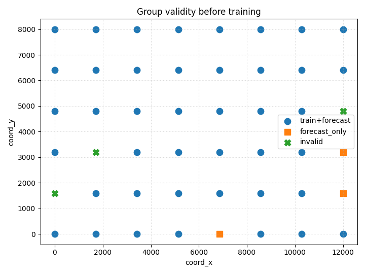
How to read this plot#
The most important interpretation is:
train+forecast: group is safe for full supervised workflow;
forecast_only: group can still support forecast-time processing, but not training;
invalid: group is too incomplete for either role.
This is exactly the kind of Stage-1 issue that should be identified before the user starts reading training curves or forecast maps.
Final takeaway#
GroupMasks makes Stage-1 validity logic explicit.
It tells the user:
which years were required,
which groups satisfy training requirements,
which groups satisfy only forecasting requirements,
and how much of the dataset survives preprocessing.
Total running time of the script: (0 minutes 0.192 seconds)