
Note
Go to the end to download the full example code.
Why physics matters in core forecasting#
This application turns the core-and-ablation comparison into a practical reading path. Instead of only showing one figure, it starts from a scientific question that a deployment team would naturally ask:
Do the physics terms change the forecast in a useful way, or do they only make the model look more sophisticated?
The page uses the reported Nansha and Zhongshan summary metrics as a compact application table. It then adds a second view that makes the trade-off between accuracy, coverage, and sharpness easier to read.
What this application shows#
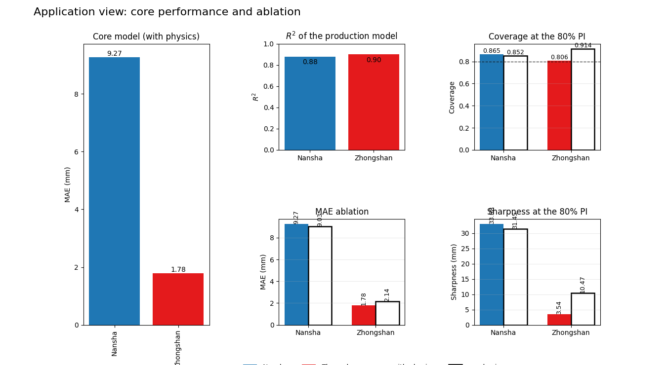
The with-physics model is strong in both basins.
The ablation must be read jointly across point error and interval behavior.
Physics is not a magic switch that wins every bar in every city; its value is that it changes the forecast in a mechanistically interpretable way and often yields a more deployment-ready uncertainty profile.
Why this matters#
A lower MAE alone is not enough for operational forecasting. Decision support also depends on whether the prediction intervals remain close to their nominal coverage and whether those intervals stay sharp enough to separate zones that may require different actions.
from __future__ import annotations

import numpy as np
import pandas as pd
import matplotlib.pyplot as plt
from matplotlib.patches import Patch

TARGET_COVERAGE = 0.80

CITY_COLORS = {
    "Nansha": "#1f77b4",
    "Zhongshan": "#e41a1c",
}


def build_application_table() -> pd.DataFrame:
    """Return the compact case-study metric table.

    The values reproduce the summary shown in the
    core-and-ablation figure and its discussion-ready metric
    labels.
    """
    rows = [
        {
            "city": "Nansha",
            "variant": "with physics",
            "r2": 0.88,
            "mae_mm": 9.27,
            "mse_mm2": 262.47,
            "coverage80": 0.865,
            "sharpness80_mm": 33.082,
        },
        {
            "city": "Nansha",
            "variant": "no physics",
            "r2": np.nan,
            "mae_mm": 9.03,
            "mse_mm2": 237.78,
            "coverage80": 0.852,
            "sharpness80_mm": 31.453,
        },
        {
            "city": "Zhongshan",
            "variant": "with physics",
            "r2": 0.90,
            "mae_mm": 1.78,
            "mse_mm2": 7.57,
            "coverage80": 0.806,
            "sharpness80_mm": 3.544,
        },
        {
            "city": "Zhongshan",
            "variant": "no physics",
            "r2": np.nan,
            "mae_mm": 2.14,
            "mse_mm2": 16.36,
            "coverage80": 0.914,
            "sharpness80_mm": 10.472,
        },
    ]
    return pd.DataFrame(rows)


def summarize_tradeoffs(df: pd.DataFrame) -> pd.DataFrame:
    """Build a city-wise application summary.

    Positive values in ``mae_gain_pct`` and ``mse_gain_pct``
    mean the with-physics variant reduces error relative to
    the no-physics variant. Positive values in
    ``sharpness_gain_mm`` mean the with-physics interval is
    narrower. Positive values in ``coverage_gain_to_target``
    mean the with-physics variant is closer to the nominal
    80%% coverage target.
    """
    rows: list[dict[str, float | str]] = []

    for city, group in df.groupby("city", sort=False):
        with_phys = group[group["variant"] == "with physics"]
        no_phys = group[group["variant"] == "no physics"]

        wp = with_phys.iloc[0]
        np_ = no_phys.iloc[0]

        rows.append(
            {
                "city": city,
                "mae_gain_pct": 100.0
                * (np_["mae_mm"] - wp["mae_mm"])
                / np_["mae_mm"],
                "mse_gain_pct": 100.0
                * (np_["mse_mm2"] - wp["mse_mm2"])
                / np_["mse_mm2"],
                "sharpness_gain_mm": (
                    np_["sharpness80_mm"]
                    - wp["sharpness80_mm"]
                ),
                "coverage_gain_to_target": (
                    abs(np_["coverage80"] - TARGET_COVERAGE)
                    - abs(wp["coverage80"] - TARGET_COVERAGE)
                ),
            }
        )

    return pd.DataFrame(rows)
Problem framing#
The role of this page is not to prove that physics must win every metric in every basin. That would be too strong, and it would also hide the scientific value of the ablation. The useful question is narrower:
does the with-physics model remain competitive in point error,
does it keep interval behavior close to the target, and
does it do so in a way that is easier to defend physically?
The compact table below is enough to discuss that question clearly before running the full script on real result folders.
metrics = build_application_table()
summary = summarize_tradeoffs(metrics)

print("Application table:\n")
print(metrics.round(3).to_string(index=False))

print("\nCity-wise trade-off summary:\n")
print(summary.round(3).to_string(index=False))
Application table:

     city      variant   r2  mae_mm  mse_mm2  coverage80  sharpness80_mm
   Nansha with physics 0.88    9.27   262.47       0.865          33.082
   Nansha   no physics  NaN    9.03   237.78       0.852          31.453
Zhongshan with physics 0.90    1.78     7.57       0.806           3.544
Zhongshan   no physics  NaN    2.14    16.36       0.914          10.472

City-wise trade-off summary:

     city  mae_gain_pct  mse_gain_pct  sharpness_gain_mm  coverage_gain_to_target
   Nansha        -2.658       -10.384             -1.629                   -0.013
Zhongshan        16.822        53.729              6.928                    0.108
Rebuild the core-and-ablation view#
We start with a compact educational reconstruction of the application figure. The first panel shows the reported performance of the production model with physics. The next panels compare the with-physics and no-physics variants on the metrics that matter most for operational reading: point error, interval coverage, and interval sharpness.
fig = plt.figure(figsize=(13.5, 7.4))
grid = fig.add_gridspec(2, 3, wspace=0.55, hspace=0.65)

ax_a = fig.add_subplot(grid[:, 0])
ax_b = fig.add_subplot(grid[0, 1])
ax_c = fig.add_subplot(grid[1, 1])
ax_d = fig.add_subplot(grid[0, 2])
ax_e = fig.add_subplot(grid[1, 2])

cities = ["Nansha", "Zhongshan"]
x = np.arange(len(cities))
width = 0.35

with_phys = (
    metrics[metrics["variant"] == "with physics"]
    .set_index("city")
    .loc[cities]
)
no_phys = (
    metrics[metrics["variant"] == "no physics"]
    .set_index("city")
    .loc[cities]
)

big_bars = ax_a.bar(
    x,
    with_phys["mae_mm"],
    color=[CITY_COLORS[c] for c in cities],
)
ax_a.set_title("Core model (with physics)")
ax_a.set_ylabel("MAE (mm)")
ax_a.set_xticks(x, cities, rotation=90)
for bar in big_bars:
    h = bar.get_height()
    ax_a.text(
        bar.get_x() + bar.get_width() / 2.0,
        h,
        f"{h:.2f}",
        ha="center",
        va="bottom",
        fontsize=10,
    )

r2_bars = ax_b.bar(
    x,
    with_phys["r2"],
    color=[CITY_COLORS[c] for c in cities],
)
ax_b.set_title(r"$R^2$ of the production model")
ax_b.set_ylabel(r"$R^2$")
ax_b.set_xticks(x, cities)
ax_b.set_ylim(0.0, 1.0)
for bar in r2_bars:
    h = bar.get_height()
    ax_b.text(
        bar.get_x() + bar.get_width() / 2.0,
        h - 0.02,
        f"{h:.2f}",
        ha="center",
        va="top",
        fontsize=10,
        color="black",
    )

for ax, metric, title, ylabel in [
    (ax_c, "mae_mm", "MAE ablation", "MAE (mm)"),
    (ax_d, "coverage80", "Coverage at the 80% PI", "Coverage"),
    (
        ax_e,
        "sharpness80_mm",
        "Sharpness at the 80% PI",
        "Sharpness (mm)",
    ),
]:
    bars_with = ax.bar(
        x - width / 2.0,
        with_phys[metric],
        width=width,
        color=[CITY_COLORS[c] for c in cities],
        label="with physics",
    )
    bars_no = ax.bar(
        x + width / 2.0,
        no_phys[metric],
        width=width,
        facecolor="none",
        edgecolor="black",
        linewidth=1.8,
        label="no physics",
    )
    ax.set_title(title)
    ax.set_ylabel(ylabel)
    ax.set_xticks(x, cities)
    ax.grid(axis="y", alpha=0.25)

    if metric == "coverage80":
        ax.axhline(
            TARGET_COVERAGE,
            color="black",
            linestyle="--",
            linewidth=1.0,
            alpha=0.7,
        )

    for bars in (bars_with, bars_no):
        for bar in bars:
            h = bar.get_height()
            ax.text(
                bar.get_x() + bar.get_width() / 2.0,
                h,
                f"{h:.3f}" if metric == "coverage80" else f"{h:.2f}",
                ha="center",
                va="bottom",
                fontsize=9,
                rotation=90 if metric != "coverage80" else 0,
            )

legend_handles = [
    Patch(facecolor=CITY_COLORS["Nansha"], label="Nansha"),
    Patch(
        facecolor=CITY_COLORS["Zhongshan"],
        label="Zhongshan",
    ),
    Patch(facecolor="black", alpha=0.0, label="with physics"),
    Patch(
        facecolor="white",
        edgecolor="black",
        linewidth=1.8,
        label="no physics",
    ),
]

fig.legend(
    handles=legend_handles,
    ncols=4,
    loc="upper center",
    bbox_to_anchor=(0.56, 0.02),
    frameon=False,
)
fig.suptitle(
    "Application view: core performance and ablation",
    x=0.05,
    ha="left",
    fontsize=16,
)
Text(0.05, 0.98, 'Application view: core performance and ablation')
Read the trade-off in decision space#
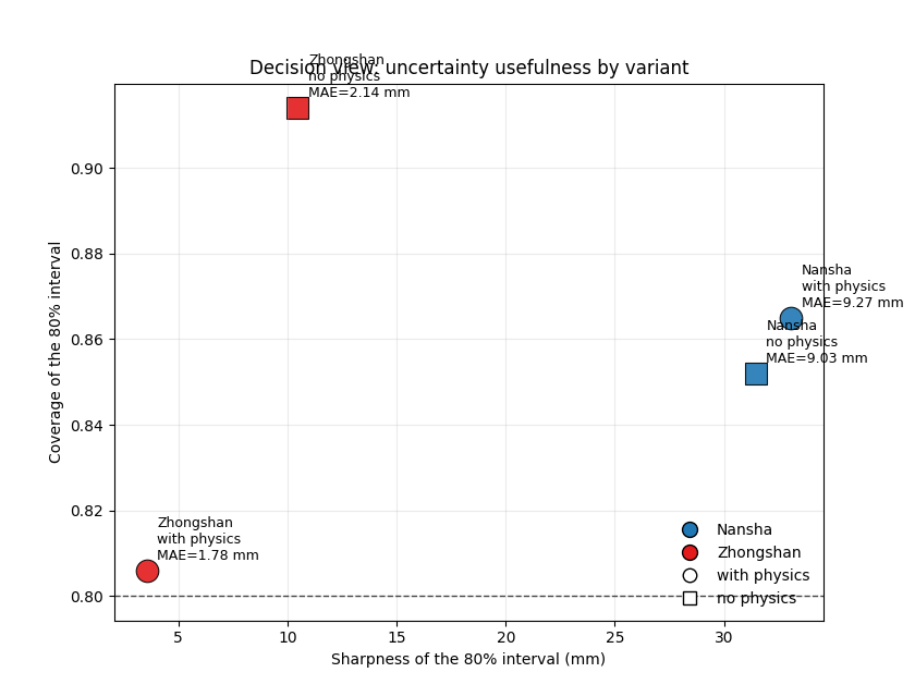
The grouped bars are useful, but a deployment reader often wants one immediate answer: which variant sits closer to a desirable operating region with high coverage, low sharpness, and low MAE?
The scatter below answers that question in one view. The horizontal axis rewards narrower intervals, the vertical axis rewards coverage close to or above the nominal target, and the annotation reports the point error directly.
The resulting pattern is informative:
In Zhongshan, physics improves both the point error and the interval usefulness, while also pulling coverage back toward the nominal 80%% target.
In Nansha, the ablation is more balanced. The no-physics variant is slightly sharper and slightly lower in point error, but the with-physics run remains close in performance while keeping the scientific interpretation on a reduced-physics scaffold.
That is exactly why this application belongs in a featured section: it shows that model choice is not only about one metric, but about the full forecast behavior that a city or basin team must defend.
fig, ax = plt.subplots(figsize=(8.4, 6.4))

markers = {
    "with physics": "o",
    "no physics": "s",
}

for row in metrics.itertuples(index=False):
    ax.scatter(
        row.sharpness80_mm,
        row.coverage80,
        s=220,
        marker=markers[row.variant],
        color=CITY_COLORS[row.city],
        edgecolor="black",
        linewidth=0.8,
        alpha=0.9,
    )

    label = (
        f"{row.city}\n"
        f"{row.variant}\n"
        f"MAE={row.mae_mm:.2f} mm"
    )
    ax.annotate(
        label,
        (row.sharpness80_mm, row.coverage80),
        xytext=(7, 7),
        textcoords="offset points",
        fontsize=9,
    )

ax.axhline(
    TARGET_COVERAGE,
    linestyle="--",
    linewidth=1.0,
    color="black",
    alpha=0.7,
)
ax.set_xlabel("Sharpness of the 80% interval (mm)")
ax.set_ylabel("Coverage of the 80% interval")
ax.set_title("Decision view: uncertainty usefulness by variant")
ax.grid(alpha=0.25)

city_handles = [
    plt.Line2D(
        [0],
        [0],
        marker="o",
        color="w",
        markerfacecolor=CITY_COLORS[city],
        markeredgecolor="black",
        markersize=10,
        label=city,
    )
    for city in cities
]

variant_handles = [
    plt.Line2D(
        [0],
        [0],
        marker=markers[variant],
        color="black",
        linestyle="None",
        markerfacecolor="white",
        markersize=9,
        label=variant,
    )
    for variant in markers
]

ax.legend(
    handles=city_handles + variant_handles,
    frameon=False,
    loc="lower right",
)
<matplotlib.legend.Legend object at 0x749e5534f320>
Practical interpretation#
Three takeaways make this page useful in practice.
First, the production model with physics is not selected because it must dominate every metric in every basin. Instead, it is selected because it remains strong while keeping the forecast attached to an auditable reduced- physics interpretation.
Second, the ablation is regime-dependent. Zhongshan shows a clear gain from physics in both error and interval quality, whereas Nansha shows a tighter trade-off. That difference is scientifically valuable because it warns the reader not to oversimplify cross-basin behavior.
Third, the page shows why GeoPrior should be read as a forecasting framework rather than a single score. The right question is not only “which MAE is lower?” but also “which variant gives a better calibrated and more useful uncertainty profile for the decisions we care about?”
From representative case study to real artifacts#
The miniature case study above is self-contained, which is ideal for a gallery page. In production, the same workflow should be fed from real result folders through the existing plotting backend.
geoprior plot core-ablation \
  --ns-with results/nansha_with_phys \
  --ns-no results/nansha_no_phys \
  --zh-with results/zhongshan_with_phys \
  --zh-no results/zhongshan_no_phys
from geoprior.scripts.plot_core_ablation import (
    collect_fig3_metrics,
    plot_fig3_core_ablation,
)

df = collect_fig3_metrics(
    cities=["Nansha", "Zhongshan"],
    ns_with="results/nansha_with_phys",
    ns_no="results/nansha_no_phys",
    zh_with="results/zhongshan_with_phys",
    zh_no="results/zhongshan_no_phys",
)

plot_fig3_core_ablation(
    df,
    cities=["Nansha", "Zhongshan"],
    core_metric="mae",
    err_metric="mse",
    out="fig3-core-ablation",
    out_csv="ext-table-fig3-metrics.csv",
    out_tex=None,
    out_xlsx=None,
    dpi=300,
    show_legend=True,
    show_labels=True,
    show_ticklabels=True,
    show_title=True,
    show_panel_titles=True,
    show_values=True,
    show_panel_labels=True,
    title=None,
)
That production call is what turns this gallery lesson into a reusable application page for new cities, retrained model variants, or updated ablation studies.
Total running time of the script: (0 minutes 0.382 seconds)