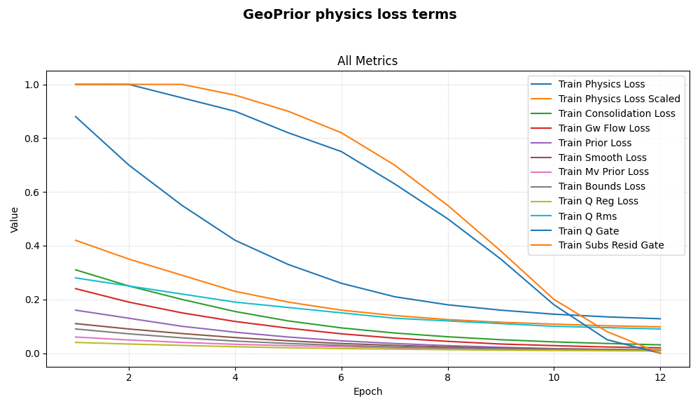
Plot physics loss terms from a GeoPrior training history

This example teaches you how to use GeoPrior’s plot_physics_losses_in helper.

Unlike the publication-oriented scripts in figure_generation/, this function is a compact model-inspection utility. It focuses only on the physics loss terms and related diagnostics stored in a training history.

Why this matters

GeoPrior histories can contain many metrics, but when you want to inspect the physics side of training, the most useful view is often a single panel containing the main physics loss terms:

• the raw and scaled physics objectives,

• PDE residual losses,

• prior and bounds penalties,

• and optional forcing diagnostics.

This helper does exactly that.

Imports

We call the real plotting helper from the package and feed it a compact synthetic history dictionary.

from __future__ import annotations

import tempfile
from pathlib import Path

import numpy as np

from geoprior.models import plot_physics_losses_in

Build a compact synthetic history

The real helper accepts a Keras History or a plain dict. For the lesson page, a plain dict is enough.

We include:

• the canonical physics loss keys used by the helper,

• a few optional diagnostics,

• unrelated keys that should be ignored by this helper,

• and one gate term that touches zero so the requested log scale can safely fall back to symlog when necessary.

epochs = np.arange(1, 13, dtype=int)

history = {
    "loss": (
        np.array(
            [2.30, 1.88, 1.53, 1.27, 1.06, 0.91,
             0.81, 0.73, 0.67, 0.63, 0.60, 0.58]
        )
    ).tolist(),
    "val_loss": (
        np.array(
            [2.48, 2.01, 1.66, 1.39, 1.19, 1.04,
             0.95, 0.88, 0.84, 0.81, 0.79, 0.78]
        )
    ).tolist(),
    "physics_loss": (
        np.array(
            [0.88, 0.70, 0.55, 0.42, 0.33, 0.26,
             0.21, 0.18, 0.16, 0.145, 0.135, 0.128]
        )
    ).tolist(),
    "physics_loss_scaled": (
        np.array(
            [0.42, 0.35, 0.29, 0.23, 0.19, 0.16,
             0.14, 0.125, 0.115, 0.108, 0.102, 0.098]
        )
    ).tolist(),
    "consolidation_loss": (
        np.array(
            [0.31, 0.25, 0.20, 0.155, 0.120, 0.094,
             0.075, 0.061, 0.050, 0.042, 0.036, 0.031]
        )
    ).tolist(),
    "gw_flow_loss": (
        np.array(
            [0.24, 0.19, 0.15, 0.118, 0.093, 0.072,
             0.056, 0.044, 0.034, 0.028, 0.023, 0.020]
        )
    ).tolist(),
    "prior_loss": (
        np.array(
            [0.16, 0.13, 0.10, 0.078, 0.060, 0.046,
             0.036, 0.028, 0.022, 0.017, 0.014, 0.012]
        )
    ).tolist(),
    "smooth_loss": (
        np.array(
            [0.11, 0.090, 0.073, 0.058, 0.046, 0.036,
             0.029, 0.023, 0.019, 0.016, 0.014, 0.012]
        )
    ).tolist(),
    "mv_prior_loss": (
        np.array(
            [0.060, 0.049, 0.040, 0.033, 0.028, 0.024,
             0.020, 0.017, 0.015, 0.013, 0.012, 0.011]
        )
    ).tolist(),
    "bounds_loss": (
        np.array(
            [0.090, 0.072, 0.057, 0.045, 0.036, 0.029,
             0.023, 0.019, 0.016, 0.014, 0.012, 0.011]
        )
    ).tolist(),
    "q_reg_loss": (
        np.array(
            [0.040, 0.034, 0.029, 0.024, 0.020, 0.017,
             0.015, 0.013, 0.011, 0.010, 0.009, 0.008]
        )
    ).tolist(),
    "q_rms": (
        np.array(
            [0.28, 0.25, 0.22, 0.19, 0.17, 0.15,
             0.13, 0.12, 0.11, 0.10, 0.095, 0.090]
        )
    ).tolist(),
    "q_gate": (
        np.array(
            [1.0, 1.0, 0.95, 0.90, 0.82, 0.75,
             0.63, 0.50, 0.35, 0.18, 0.05, 0.00]
        )
    ).tolist(),
    "subs_resid_gate": (
        np.array(
            [1.0, 1.0, 1.0, 0.96, 0.90, 0.82,
             0.70, 0.55, 0.38, 0.20, 0.08, 0.00]
        )
    ).tolist(),
}

print("History keys")
for k in history:
    print(" -", k)

History keys
 - loss
 - val_loss
 - physics_loss
 - physics_loss_scaled
 - consolidation_loss
 - gw_flow_loss
 - prior_loss
 - smooth_loss
 - mv_prior_loss
 - bounds_loss
 - q_reg_loss
 - q_rms
 - q_gate
 - subs_resid_gate

Plot the physics-loss dashboard directly

The helper automatically:

• keeps only the known physics-loss keys,

• ignores unrelated history terms,

• groups the survivors into one panel called Physics,

• and requests log-like scaling.

Because some gate values approach zero, the underlying history plotter can safely switch to symlog when needed.

plot_physics_losses_in(
    history,
    title="GeoPrior physics loss terms",
    style="default",
)

Save the physics-loss figure

When savefig has no extension, the underlying plot helper adds .png automatically.

tmp_dir = Path(
    tempfile.mkdtemp(prefix="gp_sg_plot_phys_losses_")
)
save_stem = tmp_dir / "physics_terms"

plot_physics_losses_in(
    history,
    title="Saved physics loss dashboard",
    savefig=str(save_stem),
)

saved_png = tmp_dir / "physics_terms.png"

print("")
print("Saved file")
print(" -", saved_png)

[OK] Saved figure -> /tmp/gp_sg_plot_phys_losses_lmul22ui/physics_terms.png

Saved file
 - /tmp/gp_sg_plot_phys_losses_lmul22ui/physics_terms.png

Show what the helper is selecting

The real helper uses a fixed preferred key list and then keeps only the entries that actually exist in the history.

candidate_keys = [
    "physics_loss",
    "physics_loss_scaled",
    "consolidation_loss",
    "gw_flow_loss",
    "prior_loss",
    "smooth_loss",
    "mv_prior_loss",
    "bounds_loss",
    "q_reg_loss",
    "q_rms",
    "q_gate",
    "subs_resid_gate",
]

selected = [k for k in candidate_keys if k in history]

print("")
print("Selected physics keys")
for k in selected:
    print(" -", k)

Selected physics keys
 - physics_loss
 - physics_loss_scaled
 - consolidation_loss
 - gw_flow_loss
 - prior_loss
 - smooth_loss
 - mv_prior_loss
 - bounds_loss
 - q_reg_loss
 - q_rms
 - q_gate
 - subs_resid_gate

Learn how to read the physics panel

A useful reading order is:

1. compare physics_loss and physics_loss_scaled to see how strongly the global physics objective is contributing;

2. compare consolidation_loss and gw_flow_loss to see which PDE family is dominating;

3. inspect prior_loss, smooth_loss, mv_prior_loss, and bounds_loss to see which regularizers remain active late in training;

4. inspect q_* and subs_resid_gate only when those optional diagnostics are enabled in the run.

This gives a much cleaner view than mixing these terms into a full all-metrics dashboard.

Why the raw and scaled physics losses both matter

GeoPrior logs both:

• physics_loss: the raw aggregated physics objective,

• physics_loss_scaled: the actual contribution after the offset-aware multiplier.

Looking at both helps separate:

• whether the underlying residual magnitudes are shrinking,

• from whether the optimizer is currently giving those terms a strong contribution.

Why the gate diagnostics are useful

Optional keys such as:

• q_gate

• subs_resid_gate

are not losses in the usual sense. They are control or schedule diagnostics.

But plotting them beside the other physics terms is still useful, because they help explain why a regularizer or residual family may appear to switch on, ramp up, or saturate during training.

Why this page belongs in model_inspection

This helper is not building a paper figure and it is not exporting a reusable artifact.

Its role is to inspect the internal physics side of optimization.

So it belongs naturally with the other model-inspection helpers.

A natural next lesson

The clean next page after this is autoplot_geoprior_history.py, because that helper simply automates the saving of:

• the epsilon dashboard,

• and the physics-loss dashboard.