
Note
Go to the end to download the full example code.
Compute exceedance Brier scores from calibrated forecasts#
This example teaches you how to use GeoPrior’s
brier-exceedance utility.
Unlike the plotting scripts, this command builds a tidy evaluation table. It turns calibrated forecast CSVs into exceedance Brier scores across one or more thresholds.
Why this matters#
Quantile forecasts are useful only if we can turn them into event probabilities and score those probabilities against observed events.
This builder does exactly that for subsidence exceedance events:
define an event such as
subsidence_actual >= 50 mm/yr,approximate the event probability from
q10,q50, andq90,compute the Brier score,
export the results as one tidy CSV.
That makes it a strong lesson page for the
tables_and_summaries section.
Imports#
We call the real production entrypoint from the project code. Then we read the generated CSV back in and build one compact teaching preview.
from __future__ import annotations

import tempfile
from pathlib import Path

import matplotlib.pyplot as plt
import numpy as np
import pandas as pd

from geoprior.scripts.compute_brier_exceedance import (
    brier_exceedance_main,
    exceed_prob_from_quantiles,
)
Build two compact synthetic calibrated forecast tables#
The production script expects calibrated forecast CSVs with:
coord_t
subsidence_actual
subsidence_q10
subsidence_q50
subsidence_q90
For the lesson, we build two city-level tables:
Nansha
Zhongshan
over three hold-out years:
2020
2021
2022
The synthetic data are designed so that:
Zhongshan is slightly more subsidence-prone,
uncertainty widens for larger values,
and the actuals are noisy but still broadly aligned with the forecast quantiles.
rng = np.random.default_rng(42)

years = [2020, 2021, 2022]
n_per_year = 55


def _make_city_df(
    *,
    city: str,
    level_shift: float,
    spread_scale: float,
) -> pd.DataFrame:
    rows: list[dict[str, float | int | str]] = []

    for year in years:
        yr_shift = 3.5 * (year - 2020)

        for sample_idx in range(n_per_year):
            base = 28.0 + level_shift + yr_shift
            spatial = rng.normal(0.0, 8.0)
            latent = max(1.0, base + spatial)

            width = 8.0 + spread_scale * (latent / 40.0)
            q50 = latent
            q10 = max(0.0, q50 - 1.25 * width)
            q90 = q50 + 1.25 * width

            actual = q50 + rng.normal(0.0, 0.75 * width)

            rows.append(
                {
                    "city": city,
                    "sample_idx": sample_idx,
                    "coord_t": year,
                    "subsidence_actual": float(actual),
                    "subsidence_q10": float(q10),
                    "subsidence_q50": float(q50),
                    "subsidence_q90": float(q90),
                    "subsidence_unit": "mm/yr",
                }
            )

    return pd.DataFrame(rows)


ns_df = _make_city_df(
    city="Nansha",
    level_shift=0.0,
    spread_scale=6.0,
)

zh_df = _make_city_df(
    city="Zhongshan",
    level_shift=9.0,
    spread_scale=7.0,
)

print("Nansha preview")
print(ns_df.head(6).to_string(index=False))

print("")
print("Zhongshan preview")
print(zh_df.head(6).to_string(index=False))
Nansha preview
  city  sample_idx  coord_t  subsidence_actual  subsidence_q10  subsidence_q50  subsidence_q90 subsidence_unit
Nansha           0     2020            20.6367         14.7307         30.4377         46.1448           mm/yr
Nansha           1     2020            43.2450         17.6279         34.0036         50.3793           mm/yr
Nansha           2     2020             2.7633          0.0683         12.3917         24.7152           mm/yr
Nansha           3     2020            26.0927         13.5810         29.0227         44.4645           mm/yr
Nansha           4     2020            20.0731         12.6408         27.8656         43.0904           mm/yr
Nansha           5     2020            42.7676         18.4661         35.0352         51.6043           mm/yr

Zhongshan preview
     city  sample_idx  coord_t  subsidence_actual  subsidence_q10  subsidence_q50  subsidence_q90 subsidence_unit
Zhongshan           0     2020            57.0227         28.3514         49.0898         69.8282           mm/yr
Zhongshan           1     2020            21.1473         14.5379         31.4086         48.2792           mm/yr
Zhongshan           2     2020            24.0131         19.1111         37.2623         55.4134           mm/yr
Zhongshan           3     2020            34.7983         14.7116         31.6309         48.5501           mm/yr
Zhongshan           4     2020            53.5898         26.1270         46.2425         66.3580           mm/yr
Zhongshan           5     2020            21.2417          4.5857         18.6697         32.7537           mm/yr
Write the synthetic CSV inputs#
We use explicit per-city CSVs here because the production command supports that mode directly, and it keeps the lesson independent from any external results tree.
tmp_dir = Path(
    tempfile.mkdtemp(prefix="gp_sg_brier_exceedance_")
)

ns_csv = tmp_dir / "nansha_calibrated_test.csv"
zh_csv = tmp_dir / "zhongshan_calibrated_test.csv"

ns_df.to_csv(ns_csv, index=False)
zh_df.to_csv(zh_csv, index=False)

print("")
print(f"Nansha CSV: {ns_csv}")
print(f"Zhongshan CSV: {zh_csv}")
Nansha CSV: /tmp/gp_sg_brier_exceedance_9ktcvx_c/nansha_calibrated_test.csv
Zhongshan CSV: /tmp/gp_sg_brier_exceedance_9ktcvx_c/zhongshan_calibrated_test.csv
Run the real Brier-exceedance builder#
We ask the production command to score three exceedance thresholds over the 2020–2022 hold-out years.
The output is one tidy CSV with:
city
source
years
threshold_mm_per_yr
brier_score
n_samples
src_csv
     city source          years  threshold_mm_per_yr  brier_score  n_samples                                                            src_csv
   Nansha   test 2020,2021,2022              30.0000       0.1639        165    /tmp/gp_sg_brier_exceedance_9ktcvx_c/nansha_calibrated_test.csv
   Nansha   test 2020,2021,2022              50.0000       0.0551        165    /tmp/gp_sg_brier_exceedance_9ktcvx_c/nansha_calibrated_test.csv
   Nansha   test 2020,2021,2022              70.0000       0.0190        165    /tmp/gp_sg_brier_exceedance_9ktcvx_c/nansha_calibrated_test.csv
Zhongshan   test 2020,2021,2022              30.0000       0.1441        165 /tmp/gp_sg_brier_exceedance_9ktcvx_c/zhongshan_calibrated_test.csv
Zhongshan   test 2020,2021,2022              50.0000       0.1478        165 /tmp/gp_sg_brier_exceedance_9ktcvx_c/zhongshan_calibrated_test.csv
Zhongshan   test 2020,2021,2022              70.0000       0.0332        165 /tmp/gp_sg_brier_exceedance_9ktcvx_c/zhongshan_calibrated_test.csv

[OK] brier -> /tmp/gp_sg_brier_exceedance_9ktcvx_c/brier_gallery.csv
Inspect the produced artifact#
The command writes one tidy CSV. That is the main artifact of this builder.
tab = pd.read_csv(out_csv)

print("")
print("Written file")
print(" -", out_csv.name)

print("")
print("Brier table")
print(tab.to_string(index=False))
Written file
 - brier_gallery.csv

Brier table
     city source          years  threshold_mm_per_yr  brier_score  n_samples                                                            src_csv
   Nansha   test 2020,2021,2022              30.0000       0.1639        165    /tmp/gp_sg_brier_exceedance_9ktcvx_c/nansha_calibrated_test.csv
   Nansha   test 2020,2021,2022              50.0000       0.0551        165    /tmp/gp_sg_brier_exceedance_9ktcvx_c/nansha_calibrated_test.csv
   Nansha   test 2020,2021,2022              70.0000       0.0190        165    /tmp/gp_sg_brier_exceedance_9ktcvx_c/nansha_calibrated_test.csv
Zhongshan   test 2020,2021,2022              30.0000       0.1441        165 /tmp/gp_sg_brier_exceedance_9ktcvx_c/zhongshan_calibrated_test.csv
Zhongshan   test 2020,2021,2022              50.0000       0.1478        165 /tmp/gp_sg_brier_exceedance_9ktcvx_c/zhongshan_calibrated_test.csv
Zhongshan   test 2020,2021,2022              70.0000       0.0332        165 /tmp/gp_sg_brier_exceedance_9ktcvx_c/zhongshan_calibrated_test.csv
Show how the exceedance probability is built from quantiles#
Internally, the script approximates the exceedance probability from q10, q50, and q90 using a piecewise-linear CDF.
Here we compute that probability for a small Nansha subset at a 50 mm/yr threshold so the lesson page makes the mechanism more concrete.
demo = ns_df.head(8).copy()

demo["p_exceed_50"] = exceed_prob_from_quantiles(
    demo["subsidence_q10"].to_numpy(float),
    demo["subsidence_q50"].to_numpy(float),
    demo["subsidence_q90"].to_numpy(float),
    threshold=50.0,
)

demo["event_50"] = (
    demo["subsidence_actual"].to_numpy(float) >= 50.0
).astype(int)

cols = [
    "coord_t",
    "sample_idx",
    "subsidence_actual",
    "subsidence_q10",
    "subsidence_q50",
    "subsidence_q90",
    "p_exceed_50",
    "event_50",
]

print("")
print("Probability demo at threshold = 50 mm/yr")
print(demo[cols].to_string(index=False))
Probability demo at threshold = 50 mm/yr
 coord_t  sample_idx  subsidence_actual  subsidence_q10  subsidence_q50  subsidence_q90  p_exceed_50  event_50
    2020           0            20.6367         14.7307         30.4377         46.1448       0.1000         0
    2020           1            43.2450         17.6279         34.0036         50.3793       0.1093         0
    2020           2             2.7633          0.0683         12.3917         24.7152       0.1000         0
    2020           3            26.0927         13.5810         29.0227         44.4645       0.1000         0
    2020           4            20.0731         12.6408         27.8656         43.0904       0.1000         0
    2020           5            42.7676         18.4661         35.0352         51.6043       0.1387         0
    2020           6            38.9095         13.1792         28.5282         43.8773       0.1000         0
    2020           7            23.5160         15.7888         31.7401         47.6913       0.1000         0
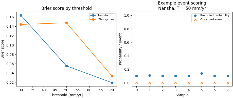
Build one compact visual preview#
This preview is not part of the production builder itself. It is a teaching aid for the gallery page.
- Left:
threshold vs Brier score by city.
- Right:
a simple calibration-style view for the 50 mm/yr event in the Nansha subset shown above.
fig, axes = plt.subplots(
    1,
    2,
    figsize=(9.2, 3.9),
    constrained_layout=True,
)

# Threshold vs Brier
ax = axes[0]
for city in ["Nansha", "Zhongshan"]:
    sub = tab.loc[tab["city"] == city].sort_values(
        "threshold_mm_per_yr"
    )
    ax.plot(
        sub["threshold_mm_per_yr"].to_numpy(float),
        sub["brier_score"].to_numpy(float),
        marker="o",
        label=city,
    )

ax.set_title("Brier score by threshold")
ax.set_xlabel("Threshold [mm/yr]")
ax.set_ylabel("Brier score")
ax.legend(fontsize=8)

# Probability vs event for a small subset
ax = axes[1]
xx = np.arange(len(demo), dtype=float)
ax.scatter(
    xx,
    demo["p_exceed_50"].to_numpy(float),
    label="Predicted probability",
)
ax.scatter(
    xx,
    demo["event_50"].to_numpy(float),
    marker="x",
    label="Observed event",
)
ax.set_title("Example event scoring\nNansha, T = 50 mm/yr")
ax.set_xlabel("Sample")
ax.set_ylabel("Probability / event")
ax.set_ylim(-0.05, 1.05)
ax.legend(fontsize=8)
<matplotlib.legend.Legend object at 0x749e55d739b0>
Learn how to read the output table#
Each row corresponds to one:
city
threshold
year selection
combination.
The most important fields are:
threshold_mm_per_yr: the event definition,brier_score: the mean squared error of the predicted event probability,n_samples: the number of valid rows used in that score.
Lower Brier is better.
What the Brier score means here#
For each threshold T, the script forms:
y = 1ifsubsidence_actual >= T,y = 0otherwise.
Then it compares:
the predicted exceedance probability
p,against the observed event indicator
y.
The Brier score is the mean of (p - y)^2 across rows.
Why the quantile interpolation matters#
This script does not assume a full parametric forecast distribution.
Instead, it uses the three available quantiles:
q10
q50
q90
to build a simple piecewise-linear approximation of the CDF. That makes the builder very practical for forecast archives that store only a few quantiles rather than full predictive samples.
Why this page uses explicit CSV inputs#
The production command can auto-discover inputs from a results tree, with:
--source auto: prefer TestSet, else fall back to Validation,--source test: require TestSet,--source val: require Validation.
In this lesson page we pass the city CSVs explicitly because it keeps the example self-contained and easy to run anywhere.
Command-line version#
The same workflow can be reproduced from the CLI.
Legacy dispatcher:
python -m scripts compute-brier-exceedance \
  --root results \
  --source auto \
  --thresholds 30,50,70 \
  --years 2020,2021,2022
Modern CLI:
geoprior build brier-exceedance \
  --root results \
  --source auto \
  --thresholds 30,50,70 \
  --years 2020,2021,2022
Explicit per-city files:
geoprior build brier-exceedance \
  --ns-csv path/to/nansha.csv \
  --zh-csv path/to/zhongshan.csv \
  --source test \
  --thresholds 30,50,70 \
  --years 2020,2021,2022 \
  --out brier_scores.csv
The gallery page teaches the builder. The command line reproduces it in a workflow.
Total running time of the script: (0 minutes 0.291 seconds)