
Note
Go to the end to download the full example code.
Inspect calibration statistics before trusting interval forecasts#
This lesson explains how to inspect the compact
calibration_stats.json artifact produced by the forecast
calibration workflow.
Why this file matters#
Calibration is easy to misunderstand. A calibration step can improve coverage while also making intervals too wide to be useful. In other words, “better calibrated” does not automatically mean “better for forecasting decisions.”
The calibration-stats artifact helps answer practical questions such as:
Was the target interval clearly defined?
Did the overall coverage move closer to the target?
Which forecast horizons required widening the intervals?
Did the long-horizon correction become too aggressive?
Was the gain in coverage paid for by a large increase in sharpness?
The goal of this page is therefore not only to call plotting helpers. It is to teach how to read calibration results step by step and decide whether the calibrated intervals are believable and still useful.
from __future__ import annotations

import json
import tempfile
from pathlib import Path
from pprint import pprint

import matplotlib.pyplot as plt
import pandas as pd

from geoprior.utils.inspect import (
    calibration_stats_factors_frame,
    calibration_stats_overall_frame,
    calibration_stats_per_horizon_frame,
    generate_calibration_stats,
    inspect_calibration_stats,
    load_calibration_stats,
    plot_calibration_boolean_summary,
    plot_calibration_factors,
    plot_calibration_overall_metrics,
    plot_calibration_per_horizon_coverage,
    plot_calibration_per_horizon_sharpness,
    summarize_calibration_stats,
)

pd.set_option("display.max_columns", 20)
pd.set_option("display.width", 100)
pd.set_option("display.float_format", lambda v: f"{v:0.6f}")

CALIBRATION_PALETTE = {
    "factors": "#4361EE",
    "overall": ["#457B9D", "#1D3557", "#F4A261", "#E76F51"],
    "coverage_before": "#6C757D",
    "coverage_after": "#2A9D8F",
    "sharp_before": "#B56576",
    "sharp_after": "#E56B6F",
    "checks": "#5E548E",
}
What this artifact is really checking#
The compact calibration-stats artifact is intentionally narrow. It does not try to replace the full interpretable evaluation JSON. Instead, it focuses on the small set of quantities that matter most when asking a calibration question:
the target interval and tolerance,
the per-horizon widening factors,
the overall coverage/sharpness before calibration,
the same quantities after calibration,
the per-horizon behaviour behind the global summary.
This is useful because interval quality is usually a trade-off. We want coverage to approach the target, but we do not want the intervals to become unnecessarily wide.
Create a realistic demo calibration artifact#
For a documentation lesson, we want a stable example that behaves like a real saved calibration file, without rerunning the full Stage-2 workflow. The generator gives us exactly that.
In this example, we intentionally let the third horizon receive the largest widening factor, because long-range forecasts are often where interval calibration struggles the most.
workdir = Path(tempfile.mkdtemp(prefix="gp_cal_stats_"))
out_dir = workdir
cal_path = out_dir / "nansha_calibration_stats.json"

generate_calibration_stats(
    cal_path,
    overrides={
        "target": 0.80,
        "tol": 0.02,
        "factors": {
            "1": 1.0,
            "2": 1.0,
            "3": 1.085,
        },
        "eval_before": {
            "coverage": 0.865,
            "sharpness": 33.08,
            "per_horizon": {
                "1": {
                    "coverage": 0.9790543662405667,
                    "sharpness": 23.244874687581664,
                },
                "2": {
                    "coverage": 0.8223728117459829,
                    "sharpness": 27.592224706985775,
                },
                "3": {
                    "coverage": 0.7935725653267621,
                    "sharpness": 48.40746668258111,
                },
            },
        },
        "eval_after": {
            "coverage": 0.806,
            "sharpness": 33.92,
            "per_horizon": {
                "1": {
                    "coverage": 0.9790543662405667,
                    "sharpness": 23.244874687581664,
                },
                "2": {
                    "coverage": 0.8223728117459829,
                    "sharpness": 27.592224706985775,
                },
                "3": {
                    "coverage": 0.8010410698701166,
                    "sharpness": 50.89692692253824,
                },
            },
        },
    },
)

print("Written calibration file")
print(f" - {cal_path}")
Written calibration file
 - /tmp/gp_cal_stats_lvl72pgz/nansha_calibration_stats.json
Load the artifact with the real reader#
The loader is designed to accept both a direct calibration-stats JSON and the richer interpretable evaluation JSON that embeds the same block. For the first pass, we use the direct file because it is the cleanest way to understand the structure.
cal_record = load_calibration_stats(cal_path)

print("\nArtifact header")
pprint(
    {
        "kind": cal_record.kind,
        "city": cal_record.city,
        "model": cal_record.model,
        "path": str(cal_record.path),
        "meta": cal_record.meta,
    }
)
Artifact header
{'city': None,
 'kind': 'calibration_stats',
 'meta': {'has_eval_after': True,
          'has_eval_before': True,
          'has_factors': True,
          'n_top_keys': 9,
          'source_name': 'nansha_calibration_stats.json',
          'top_keys': ['target',
                       'interval',
                       'f_max',
                       'tol',
                       'overall_key',
                       'factors_source',
                       'factors',
                       'eval_before',
                       'eval_after']},
 'model': None,
 'path': '/tmp/gp_cal_stats_lvl72pgz/nansha_calibration_stats.json'}
Start with the compact summary#
A good inspection habit is to read the semantic summary before you look at individual horizons. This answers the first decision question:
Did calibration move the overall interval behaviour in the right direction?
summary = summarize_calibration_stats(cal_record)

print("\nCompact summary")
print(json.dumps(summary, indent=2))
Compact summary
{
  "target": 0.8,
  "interval_low": 0.1,
  "interval_high": 0.9,
  "tol": 0.02,
  "n_horizons": 3,
  "factors_source": "fit",
  "coverage_before": 0.865,
  "coverage_after": 0.806,
  "sharpness_before": 33.08,
  "sharpness_after": 33.92,
  "coverage_error_before": 0.06499999999999995,
  "coverage_error_after": 0.006000000000000005,
  "coverage_error_improved": true,
  "target_reached_after": true,
  "max_factor": 1.085,
  "min_factor": 1.0,
  "has_eval_before": true,
  "has_eval_after": true,
  "has_factors": true,
  "skipped": false
}
Read the main tidy tables#
The helper frames turn the nested JSON into compact views that are easier to reason about than the raw payload.
We use three levels of reading:
the factor table,
the overall before/after table,
the per-horizon tables.
factors = calibration_stats_factors_frame(cal_record)
overall = calibration_stats_overall_frame(cal_record)
per_before = calibration_stats_per_horizon_frame(
    cal_record,
    which="eval_before",
)
per_after = calibration_stats_per_horizon_frame(
    cal_record,
    which="eval_after",
)

print("\nPer-horizon calibration factors")
print(factors)

print("\nOverall before/after metrics")
print(overall)

print("\nPer-horizon coverage and sharpness before calibration")
print(per_before)

print("\nPer-horizon coverage and sharpness after calibration")
print(per_after)
Per-horizon calibration factors
  horizon   factor
0       1 1.000000
1       2 1.000000
2       3 1.085000

Overall before/after metrics
         which  coverage  sharpness  coverage_error
0  eval_before  0.865000  33.080000        0.065000
1   eval_after  0.806000  33.920000        0.006000

Per-horizon coverage and sharpness before calibration
         which horizon  coverage  sharpness
0  eval_before       1  0.979054  23.244875
1  eval_before       2  0.822373  27.592225
2  eval_before       3  0.793573  48.407467

Per-horizon coverage and sharpness after calibration
        which horizon  coverage  sharpness
0  eval_after       1  0.979054  23.244875
1  eval_after       2  0.822373  27.592225
2  eval_after       3  0.801041  50.896927
Interpret the overall table#
The most useful first comparison is the distance to the target
coverage. The calibration summary already computes
coverage_error_before and coverage_error_after, but it is
worth making that comparison explicit in the lesson.
Here the target is 0.80. So:
a coverage of 0.865 means the uncalibrated intervals were too conservative overall,
a coverage of 0.806 is much closer to the target,
but sharpness also became larger, which means the intervals got wider.
That is the core calibration trade-off.
overall_view = overall.copy()
overall_view["target"] = summary["target"]
overall_view["distance_to_target"] = (
    overall_view["coverage"] - summary["target"]
).abs()

print("\nOverall interpretation table")
print(overall_view)
Overall interpretation table
         which  coverage  sharpness  coverage_error   target  distance_to_target
0  eval_before  0.865000  33.080000        0.065000 0.800000            0.065000
1   eval_after  0.806000  33.920000        0.006000 0.800000            0.006000
Compare horizons directly#
Global coverage can hide where the correction really happened. Per-horizon inspection often reveals that the calibration step was almost inactive at short horizons and mainly widened the uncertain tail.
horizon_compare = per_before.merge(
    per_after,
    on="horizon",
    suffixes=("_before", "_after"),
)
horizon_compare["coverage_delta"] = (
    horizon_compare["coverage_after"]
    - horizon_compare["coverage_before"]
)
horizon_compare["sharpness_delta"] = (
    horizon_compare["sharpness_after"]
    - horizon_compare["sharpness_before"]
)
horizon_compare["coverage_error_before"] = (
    horizon_compare["coverage_before"] - summary["target"]
).abs()
horizon_compare["coverage_error_after"] = (
    horizon_compare["coverage_after"] - summary["target"]
).abs()

print("\nPer-horizon comparison")
print(
    horizon_compare.loc[
        :,
        [
            "horizon",
            "coverage_before",
            "coverage_after",
            "coverage_delta",
            "coverage_error_before",
            "coverage_error_after",
            "sharpness_before",
            "sharpness_after",
            "sharpness_delta",
        ],
    ]
)
Per-horizon comparison
  horizon  coverage_before  coverage_after  coverage_delta  coverage_error_before  \
0       1         0.979054        0.979054        0.000000               0.179054
1       2         0.822373        0.822373        0.000000               0.022373
2       3         0.793573        0.801041        0.007469               0.006427

   coverage_error_after  sharpness_before  sharpness_after  sharpness_delta
0              0.179054         23.244875        23.244875         0.000000
1              0.022373         27.592225        27.592225         0.000000
2              0.001041         48.407467        50.896927         2.489460
How to read the factor table#
Calibration factors are one of the easiest places to make a wrong decision.
A factor near 1.0 means the interval was left essentially unchanged. A larger factor means the interval had to be widened.
This does not mean a larger factor is always bad. It simply means that horizon needed more correction. The real question is whether the correction improved coverage enough to justify the extra width.
In this demo:
H1 and H2 stay at 1.0, so they were already acceptable,
H3 is widened, which is consistent with it being the hardest horizon to calibrate.
print("\nFactor reading note")
if not factors.empty:
    worst = factors.loc[factors["factor"].idxmax()]
    print(
        f"Largest widening factor: H{worst['horizon']} -> "
        f"{worst['factor']:.3f}"
    )
Factor reading note
Largest widening factor: H3 -> 1.085
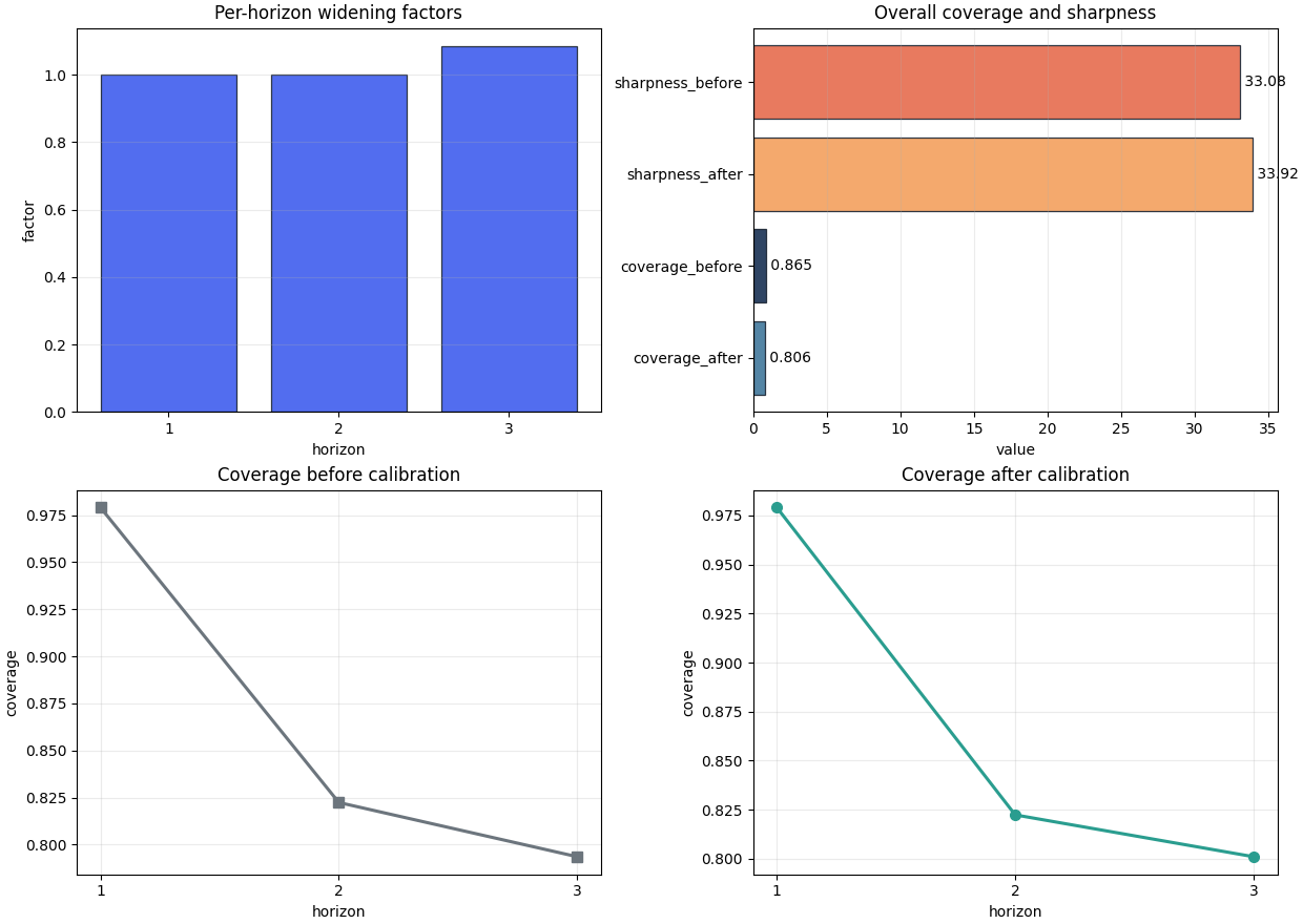
Plot the main calibration views#
A compact first inspection usually benefits from four plots:
the widening factors,
the overall before/after coverage and sharpness,
per-horizon coverage before calibration,
per-horizon coverage after calibration.
This figure helps answer:
Where did calibration act, and did it move the empirical coverage toward the target?
fig, axes = plt.subplots(
    2,
    2,
    figsize=(12.4, 8.8),
    constrained_layout=True,
)

plot_calibration_factors(
    axes[0, 0],
    cal_record,
    title="Per-horizon widening factors",
    color=CALIBRATION_PALETTE["factors"],
    edgecolor="#1F2937",
    linewidth=0.9,
    alpha=0.92,
)
plot_calibration_overall_metrics(
    axes[0, 1],
    cal_record,
    title="Overall coverage and sharpness",
    color=CALIBRATION_PALETTE["overall"],
    edgecolor="#1F2937",
    linewidth=0.9,
    alpha=0.92,
)
plot_calibration_per_horizon_coverage(
    axes[1, 0],
    cal_record,
    which="eval_before",
    title="Coverage before calibration",
    color=CALIBRATION_PALETTE["coverage_before"],
    marker="s",
    linewidth=2.2,
    markersize=7,
)
plot_calibration_per_horizon_coverage(
    axes[1, 1],
    cal_record,
    which="eval_after",
    title="Coverage after calibration",
    color=CALIBRATION_PALETTE["coverage_after"],
    marker="o",
    linewidth=2.2,
    markersize=7,
)
<Axes: title={'center': 'Coverage after calibration'}, xlabel='horizon', ylabel='coverage'>
How to interpret the first figure#
When reading the first figure, look for the following pattern:
are factors concentrated on the harder horizons?
does the post-calibration coverage move closer to the target?
does the correction stay moderate rather than explosive?
In this demo, the main action is at H3. That is exactly the kind of pattern we usually expect when uncertainty grows with horizon.
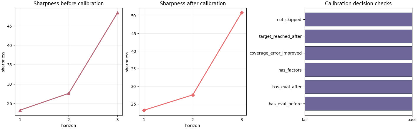
Plot the width trade-off directly#
Coverage alone is never enough. The second figure focuses on the cost of calibration in terms of interval width and on the final pass/ fail-style checks.
fig, axes = plt.subplots(
    1,
    3,
    figsize=(14.2, 4.4),
    constrained_layout=True,
)

plot_calibration_per_horizon_sharpness(
    axes[0],
    cal_record,
    which="eval_before",
    title="Sharpness before calibration",
    color=CALIBRATION_PALETTE["sharp_before"],
    marker="^",
    linewidth=2.2,
    markersize=7,
)
plot_calibration_per_horizon_sharpness(
    axes[1],
    cal_record,
    which="eval_after",
    title="Sharpness after calibration",
    color=CALIBRATION_PALETTE["sharp_after"],
    marker="D",
    linewidth=2.2,
    markersize=6.5,
)
plot_calibration_boolean_summary(
    axes[2],
    cal_record,
    title="Calibration decision checks",
    color=CALIBRATION_PALETTE["checks"],
    edgecolor="#1F2937",
    linewidth=0.8,
    alpha=0.9,
)
<Axes: title={'center': 'Calibration decision checks'}>
Read the sharpness plots with care#
A larger sharpness value means a wider interval. In many workflows, that is the hidden price of achieving better calibration.
The right question is therefore not:
Did sharpness increase?
but:
Did sharpness increase by an amount that is acceptable given the gain in coverage?
In this demo the widening is concentrated at H3. That is plausible, because the later horizon needed the strongest factor adjustment.
Use the all-in-one inspection bundle#
inspect_calibration_stats(...) is handy when you want the raw
payload, the semantic summary, and the main tidy frames in one place.
Inspector bundle keys
['factors', 'overall', 'payload', 'per_horizon_after', 'per_horizon_before', 'summary']
The module also understands the nested eval-style structure#
A useful design detail of this inspector is that it can also read the calibration block when it is embedded inside the richer interpretable evaluation JSON. This means a user can inspect calibration even when they only have the larger eval artifact at hand.
eval_like_path = out_dir / "nansha_eval_interpretable.json"
eval_like_payload = {
    "city": "nansha",
    "model": "GeoPriorSubsNet",
    "interval_calibration": {
        "factors_per_horizon_from_cal_stats": bundle["payload"],
        "factors_per_horizon": {
            row["horizon"]: row["factor"]
            for _, row in bundle["factors"].iterrows()
        },
    },
}
eval_like_path.write_text(
    json.dumps(eval_like_payload, indent=2),
    encoding="utf-8",
)

nested_record = load_calibration_stats(eval_like_path)
nested_summary = summarize_calibration_stats(nested_record)

print("\nNested eval-style summary")
print(json.dumps(nested_summary, indent=2))
Nested eval-style summary
{
  "target": 0.8,
  "interval_low": 0.1,
  "interval_high": 0.9,
  "tol": 0.02,
  "n_horizons": 3,
  "factors_source": "fit",
  "coverage_before": 0.865,
  "coverage_after": 0.806,
  "sharpness_before": 33.08,
  "sharpness_after": 33.92,
  "coverage_error_before": 0.06499999999999995,
  "coverage_error_after": 0.006000000000000005,
  "coverage_error_improved": true,
  "target_reached_after": true,
  "max_factor": 1.085,
  "min_factor": 1.0,
  "has_eval_before": true,
  "has_eval_after": true,
  "has_factors": true,
  "skipped": false
}
A practical decision rule#
For this artifact family, a reasonable quick decision rule is:
the file contains both before and after evaluation blocks,
the calibration factors are present,
the post-calibration coverage error improved,
the post-calibration coverage is within tolerance of the target,
and the largest widening factor is still interpretable.
That last part is domain-dependent. There is no universal numeric threshold, but extremely large factors are a warning sign that the forecast distribution may have been badly mis-scaled upstream.
max_factor = summary.get("max_factor")
structurally_ready = all(
    bool(summary.get(name, False))
    for name in [
        "has_eval_before",
        "has_eval_after",
        "has_factors",
        "coverage_error_improved",
        "target_reached_after",
    ]
)
moderate_factors = (
    max_factor is not None and float(max_factor) <= 2.0
)

print("\nDecision note")
if structurally_ready and moderate_factors:
    print(
        "This demo calibration artifact looks healthy enough to trust "
        "the calibrated intervals in later evaluation and reporting."
    )
elif structurally_ready:
    print(
        "Calibration improved the target fit, but the widening factors "
        "deserve a closer look before you rely on the result."
    )
else:
    print(
        "This calibration result needs attention before you use the "
        "calibrated intervals downstream."
    )
Decision note
This demo calibration artifact looks healthy enough to trust the calibrated intervals in later evaluation and reporting.
Final checklist for real workflow review#
When you inspect your own saved calibration artifact, try to answer these questions in order:
Is the target interval the one I intended to calibrate?
Did overall coverage move toward the target?
Which horizons needed the correction?
Did the width increase stay concentrated on the difficult cases?
Are the factors still small enough to remain believable?
If the answer is mostly yes, the calibration step is doing something useful. If not, the right fix may be upstream in the forecast model, not in the calibration layer itself.
Total running time of the script: (0 minutes 0.642 seconds)