
Note
Go to the end to download the full example code.
Inspect interpretable evaluation physics before reporting results#
This lesson explains how to inspect the richer
eval_physics artifact.
Compared with the compact eval_diagnostics JSON,
this artifact is broader and more interpretive. It brings
forecast skill and physics consistency into the same view.
That makes it one of the most useful files to inspect when
we want to answer questions such as:
Is the forecast reasonably accurate?
Are the physics residuals small enough to inspire trust?
Did interval calibration improve coverage?
Did that improvement come at a sharpness cost?
Are the units explicit enough for reporting and comparison?
The goal of this page is not only to call plotting helpers. It is to teach how to read the artifact like a workflow checkpoint before using the results in analysis, figures, or downstream decisions.
from __future__ import annotations

import json
import tempfile
from pathlib import Path
from pprint import pprint

import matplotlib.pyplot as plt
import pandas as pd

from geoprior.utils.inspect import (
    eval_physics_calibration_frame,
    eval_physics_calibration_per_horizon_frame,
    eval_physics_censor_frame,
    eval_physics_metrics_frame,
    eval_physics_per_horizon_frame,
    eval_physics_point_metrics_frame,
    eval_physics_units_frame,
    generate_eval_physics,
    inspect_eval_physics,
    load_eval_physics,
    plot_eval_physics_boolean_summary,
    plot_eval_physics_calibration_factors,
    plot_eval_physics_epsilons,
    plot_eval_physics_metrics,
    plot_eval_physics_per_horizon_metrics,
    plot_eval_physics_point_metrics,
    summarize_eval_physics,
)

pd.set_option("display.max_columns", 30)
pd.set_option("display.width", 108)

EVAL_PHYSICS_PALETTE = {
    "metrics": [
        "#264653", "#2A9D8F", "#8AB17D", "#E9C46A",
        "#F4A261", "#E76F51", "#B56576", "#6D597A",
        "#577590", "#277DA1", "#4D908E", "#90BE6D",
        "#F9844A", "#F94144"
    ],
    "eps": ["#355070", "#6D597A", "#B56576", "#E56B6F", "#EAAC8B"],
    "point": ["#118AB2", "#06D6A0", "#FFD166", "#EF476F"],
    "mae_line": "#C1121F",
    "cal_line": "#3A86FF",
    "r2_line": "#2A9D8F",
    "checks": "#5E548E",
}
Why this artifact matters#
The compact evaluation diagnostics file is excellent for a quick
view of forecast quality. The richer eval_physics artifact,
however, answers a broader question:
Can we trust the evaluation not only as a forecasting result, but also as a physics-aware model outcome?
This matters because a physically guided model can fail in several different ways:
forecast metrics may look acceptable while physics residuals are large,
calibration may improve coverage while intervals become too wide,
units may be unclear enough to confuse later reporting,
point accuracy may hide that later horizons degrade sharply.
So this file is best read as a decision layer between a raw run and a scientific interpretation.
Create a realistic demo artifact#
For documentation pages we want a stable artifact that looks like the real interpretable evaluation JSON, without rerunning the whole Stage-2 path. The generation helper gives us exactly that.
We deliberately keep the payload realistic:
forecast errors are non-zero,
physics losses are tiny but present,
calibration improves coverage slightly,
later horizons are harder than earlier ones,
units are explicit.
out_dir = Path(tempfile.mkdtemp(prefix="gp_eval_phys_"))
artifact_path = out_dir / "geoprior_eval_phys_demo_interpretable.json"

generate_eval_physics(
    output_path=artifact_path,
    overrides={
        "city": "nansha",
        "model": "GeoPriorSubsNet",
        "timestamp": "2026-03-29T15:23:48Z",
        "horizon": 3,
        "batch_size": 64,
        "units": {
            "subs_metrics_unit": "mm",
            "time_units": "year",
            "seconds_per_time_unit": 31556952.0,
            "epsilon_cons_raw_unit": "mm/year",
            "epsilon_gw_raw_unit": "1/year",
        },
    },
)

print("Written eval-physics artifact")
print(f" - {artifact_path}")
Written eval-physics artifact
 - /tmp/gp_eval_phys_pf3dkygd/geoprior_eval_phys_demo_interpretable.json
Load the artifact with the real reader#
Even in a lesson, it is good practice to go through the same
entry point a user would use for a real file written under
results/....
record = load_eval_physics(artifact_path)

print("\nArtifact header")
pprint(
    {
        "kind": record.kind,
        "stage": record.stage,
        "city": record.city,
        "model": record.model,
        "path": str(record.path),
    }
)
Artifact header
{'city': 'nansha',
 'kind': 'eval_physics',
 'model': 'GeoPriorSubsNet',
 'path': '/tmp/gp_eval_phys_pf3dkygd/geoprior_eval_phys_demo_interpretable.json',
 'stage': None}
Start with the semantic summary#
The summary is the best first stop because it compresses the nested artifact into a few interpretable blocks:
brief: run identity,core_metrics: forecast and loss scalars,physics: epsilon diagnostics and scaling knobs,calibration: before/after interval behavior,units: reporting conventions,checks: fast structural decision tests.
When this summary already looks suspicious, the rest of the artifact deserves closer review before any reporting step.
summary = summarize_eval_physics(record)

print("\nCompact semantic summary")
print(json.dumps(summary, indent=2))
Compact semantic summary
{
  "brief": {
    "kind": "eval_physics",
    "timestamp": "2026-03-29T15:23:48Z",
    "city": "nansha",
    "model": "GeoPriorSubsNet",
    "horizon": 3,
    "batch_size": 64,
    "quantiles": [
      0.1,
      0.5,
      0.9
    ]
  },
  "core_metrics": {
    "subs_mae_q50": 30.37,
    "subs_rmse_q50": 65.93,
    "gwl_mae_q50": 0.239,
    "gwl_rmse_q50": 0.277,
    "loss": 0.1577,
    "data_loss": 0.1577,
    "physics_loss": 4.14e-09,
    "physics_loss_scaled": 4.14e-09,
    "point_mae": 9.27,
    "point_rmse": 16.2,
    "point_r2": 0.883
  },
  "physics": {
    "epsilon_prior": 0.000354,
    "epsilon_cons": 2.11e-06,
    "epsilon_gw": 1.18e-07,
    "epsilon_cons_raw": 0.0125,
    "epsilon_gw_raw": 3.94e-06,
    "lambda_offset": 1.0,
    "physics_mult": 1.0
  },
  "calibration": {
    "target": 0.8,
    "coverage80_uncalibrated": 0.813,
    "coverage80_calibrated": 0.865,
    "sharpness80_uncalibrated": 0.0278,
    "sharpness80_calibrated": 0.0331,
    "coverage_before": 0.865,
    "coverage_after": 0.867,
    "sharpness_before": 33.08,
    "sharpness_after": 33.38,
    "factor_min": 1.0,
    "factor_max": 1.018
  },
  "units": {
    "subs_metrics_unit": "mm",
    "time_units": "year",
    "epsilon_cons_raw_unit": "mm/year",
    "epsilon_gw_raw_unit": "1/year"
  },
  "checks": {
    "has_metrics_evaluate": true,
    "has_physics_diagnostics": true,
    "has_interval_calibration": true,
    "has_point_metrics": true,
    "has_units": true,
    "has_per_horizon": true,
    "has_quantiles": true,
    "physics_loss_nonnegative": true,
    "epsilons_present": true,
    "calibration_target_in_01": true,
    "coverage_improves_or_matches": true,
    "reported_unit_present": true
  }
}
Convert the nested sections into tidy tables#
The artifact is rich, but JSON nesting is not always easy to read. The frame helpers expose the parts we usually inspect first.
metrics_frame = eval_physics_metrics_frame(record)
point_frame = eval_physics_point_metrics_frame(record)
units_frame = eval_physics_units_frame(record)
censor_frame = eval_physics_censor_frame(record)
per_h_frame = eval_physics_per_horizon_frame(record)
cal_frame = eval_physics_calibration_frame(record)
cal_per_h_frame = eval_physics_calibration_per_horizon_frame(record)

print("\nmetrics_evaluate (first rows)")
print(metrics_frame.head(18))

print("\nPoint metrics")
print(point_frame)

print("\nUnits metadata")
print(units_frame)

print("\nCensor-stratified metrics")
print(censor_frame)

print("\nPer-horizon metrics")
print(per_h_frame)

print("\nCalibration summary")
print(cal_frame)

print("\nCalibration per horizon")
print(cal_per_h_frame)
metrics_evaluate (first rows)
             section               metric    value
0   metrics_evaluate          bounds_loss 0.000000
1   metrics_evaluate   consolidation_loss 0.000000
2   metrics_evaluate            data_loss 0.157700
3   metrics_evaluate         epsilon_cons 0.000002
4   metrics_evaluate     epsilon_cons_raw 0.012500
5   metrics_evaluate           epsilon_gw 0.000000
6   metrics_evaluate       epsilon_gw_raw 0.000004
7   metrics_evaluate        epsilon_prior 0.000354
8   metrics_evaluate         gw_flow_loss 0.000000
9   metrics_evaluate     gwl_pred_mae_q50 0.239000
10  metrics_evaluate     gwl_pred_mse_q50 0.076800
11  metrics_evaluate    gwl_pred_rmse_q50 0.277000
12  metrics_evaluate        lambda_offset 1.000000
13  metrics_evaluate                 loss 0.157700
14  metrics_evaluate        mv_prior_loss 0.000000
15  metrics_evaluate         physics_loss 0.000000
16  metrics_evaluate  physics_loss_scaled 0.000000
17  metrics_evaluate         physics_mult 1.000000

Point metrics
         section metric      value
0  point_metrics    mae   9.270000
1  point_metrics    mse 262.470000
2  point_metrics     r2   0.883000
3  point_metrics   rmse  16.200000

Units metadata
                      key           value  is_numeric
0         subs_unit_to_si        0.001000        True
1  subs_factor_si_to_real     1000.000000        True
2       subs_metrics_unit              mm       False
3              time_units            year       False
4   seconds_per_time_unit 31556952.000000        True
5   epsilon_cons_raw_unit         mm/year       False
6     epsilon_gw_raw_unit          1/year       False

Censor-stratified metrics
              key                    value  is_numeric
0       flag_name  soil_thickness_censored       False
1       threshold                 0.500000        True
2    mae_censored                 0.000000        True
3  mae_uncensored                 9.270000        True

Per-horizon metrics
  metric horizon     value
0    mae      H1  3.520000
1    mae      H2  8.310000
2    mae      H3 15.980000
3     r2      H1  0.896000
4     r2      H2  0.888000
5     r2      H3  0.874000

Calibration summary
                 section                         metric     value
0   interval_calibration                cal_stats.f_max  5.000000
1   interval_calibration               cal_stats.target  0.800000
2   interval_calibration                  cal_stats.tol  0.020000
3   interval_calibration          coverage80_calibrated  0.865000
4   interval_calibration     coverage80_calibrated_phys  0.865000
5   interval_calibration        coverage80_uncalibrated  0.813000
6   interval_calibration   coverage80_uncalibrated_phys  0.813000
7   interval_calibration            eval_after.coverage  0.867000
8   interval_calibration           eval_after.sharpness 33.380000
9   interval_calibration           eval_before.coverage  0.865000
10  interval_calibration          eval_before.sharpness 33.080000
11  interval_calibration         sharpness80_calibrated  0.033100
12  interval_calibration    sharpness80_calibrated_phys 33.080000
13  interval_calibration       sharpness80_uncalibrated  0.027800
14  interval_calibration  sharpness80_uncalibrated_phys 27.820000
15  interval_calibration                         target  0.800000

Calibration per horizon
  horizon   factor  coverage_before  coverage_after  sharpness_before  sharpness_after
0       1 1.000000         0.979000        0.979000         23.240000        23.240000
1       2 1.000000         0.822000        0.822000         27.590000        27.590000
2       3 1.018000         0.794000        0.800000         48.410000        49.300000
Read the three most important blocks first#
In practice, a user usually wants to interpret this artifact in three passes.
- First pass: forecast quality
Look at MAE, RMSE, coverage, sharpness, and point metrics.
- Second pass: physics consistency
Look at
epsilon_prior,epsilon_cons, andepsilon_gwtogether with the raw epsilon quantities.- Third pass: interval usefulness
Look at calibration target, factors, coverage changes, and the sharpness penalty after calibration.
A common mistake is to look only at one of these layers. A run can look good from one angle and weak from another.
Reading pass 1: forecast quality
{'data_loss': 0.1577,
 'gwl_mae_q50': 0.239,
 'gwl_rmse_q50': 0.277,
 'loss': 0.1577,
 'physics_loss': 4.14e-09,
 'physics_loss_scaled': 4.14e-09,
 'point_mae': 9.27,
 'point_r2': 0.883,
 'point_rmse': 16.2,
 'subs_mae_q50': 30.37,
 'subs_rmse_q50': 65.93}

Reading pass 2: physics consistency
{'epsilon_cons': 2.11e-06,
 'epsilon_cons_raw': 0.0125,
 'epsilon_gw': 1.18e-07,
 'epsilon_gw_raw': 3.94e-06,
 'epsilon_prior': 0.000354,
 'lambda_offset': 1.0,
 'physics_mult': 1.0}

Reading pass 3: calibration behavior
{'coverage80_calibrated': 0.865,
 'coverage80_uncalibrated': 0.813,
 'coverage_after': 0.867,
 'coverage_before': 0.865,
 'factor_max': 1.018,
 'factor_min': 1.0,
 'sharpness80_calibrated': 0.0331,
 'sharpness80_uncalibrated': 0.0278,
 'sharpness_after': 33.38,
 'sharpness_before': 33.08,
 'target': 0.8}
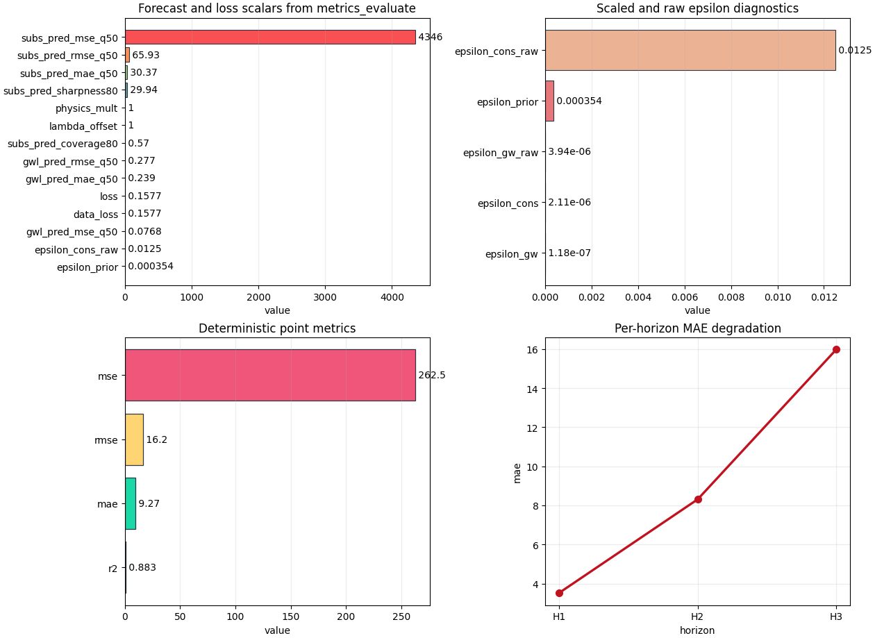
Interpret the forecast-and-loss overview#
The first plot gathers many values from metrics_evaluate.
Do not read it as a single ranking. Instead, separate it mentally
into three groups:
forecast quality -
subs_pred_mae_q50-subs_pred_rmse_q50-gwl_pred_mae_q50-gwl_pred_rmse_q50objective composition -
loss-data_loss-physics_loss-physics_loss_scaledoptimization/control scalars -
physics_mult-lambda_offset- any gate-like values.
A healthy pattern is often:
data loss dominates the total objective,
physics loss is present but not exploding,
the control scalars are finite and interpretable.
fig, axes = plt.subplots(
    2,
    2,
    figsize=(12.6, 9.2),
    constrained_layout=True,
)

plot_eval_physics_metrics(
    record,
    ax=axes[0, 0],
    title="Forecast and loss scalars from metrics_evaluate",
    color=EVAL_PHYSICS_PALETTE["metrics"],
    edgecolor="#1F2937",
    linewidth=0.8,
    alpha=0.92,
)

# Interpret the epsilon panel
# ---------------------------
#
# The epsilon plot is one of the most important parts of this lesson.
# It combines scaled and raw residual-style diagnostics.
#
# A careful reading rule is:
#
# - ``epsilon_prior`` tells us whether the closure/timescale prior is
#   internally consistent,
# - ``epsilon_cons`` tells us how well the consolidation relation is
#   respected,
# - ``epsilon_gw`` tells us how well the groundwater equation is
#   respected,
# - the corresponding raw values help us remember that "small" is
#   unit- and scaling-dependent.
#
# In other words, the scaled epsilons are convenient for model review,
# while the raw ones preserve some physical interpretability.

plot_eval_physics_epsilons(
    record,
    ax=axes[0, 1],
    title="Scaled and raw epsilon diagnostics",
    color=EVAL_PHYSICS_PALETTE["eps"],
    edgecolor="#1F2937",
    linewidth=0.8,
    alpha=0.92,
)

# Interpret point metrics
# -----------------------
#
# Point metrics are useful because they collapse the uncertainty-aware
# prediction into a simple deterministic view.
#
# This is the easiest panel for many readers, but it should not be the
# only one we trust. A model can have acceptable point MAE and still be
# poorly calibrated or physically inconsistent.

plot_eval_physics_point_metrics(
    record,
    ax=axes[1, 0],
    title="Deterministic point metrics",
    color=EVAL_PHYSICS_PALETTE["point"],
    edgecolor="#1F2937",
    linewidth=0.9,
    alpha=0.92,
)

# Interpret per-horizon degradation
# ---------------------------------
#
# The per-horizon panel is where we ask whether the run remains useful
# farther into the future.
#
# A common and acceptable pattern is that later horizons degrade.
# What matters is *how fast* they degrade. If H1 is good and H3 is much
# worse, the model may still be operational for short-range forecasting
# but not for longer-range reporting.

plot_eval_physics_per_horizon_metrics(
    record,
    metric="mae",
    ax=axes[1, 1],
    title="Per-horizon MAE degradation",
    color=EVAL_PHYSICS_PALETTE["mae_line"],
    marker="o",
    linewidth=2.4,
    markersize=7,
)

plt.show()
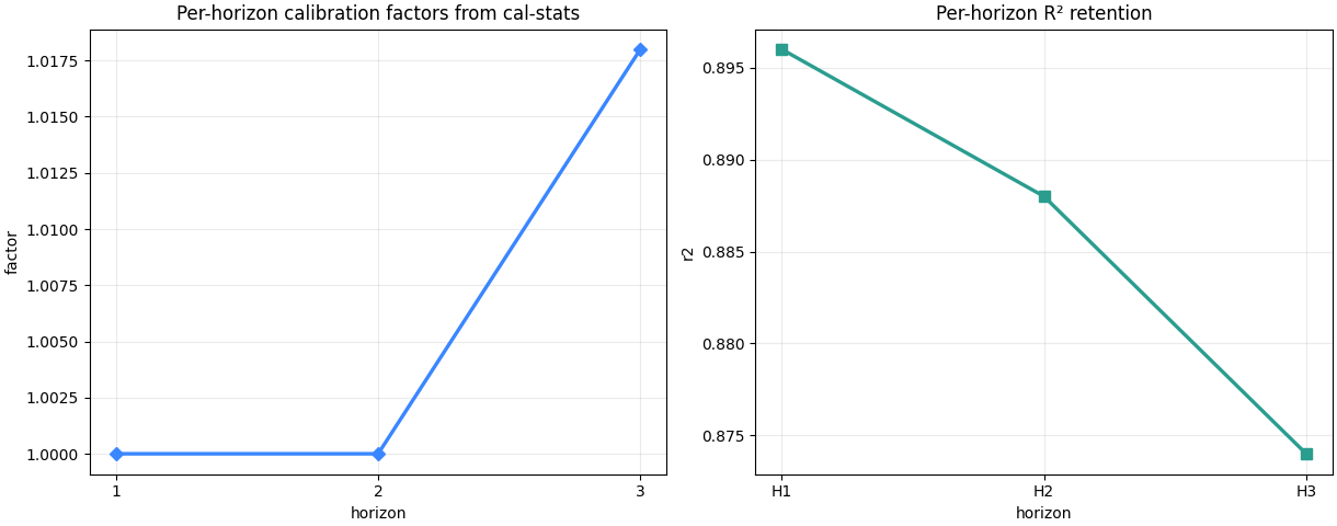
Inspect calibration separately#
Interval calibration deserves its own figure because it is not enough to say “coverage improved”. We also need to know whether the interval widening factor became excessive.
Read the factor plot like this:
factors near 1.0 mean only small adjustment,
larger factors mean stronger widening,
a late-horizon spike often means uncertainty was under-estimated farther into the forecast.
This is often acceptable, but it should make us check sharpness very carefully.
fig, axes = plt.subplots(
    1,
    2,
    figsize=(12.2, 4.8),
    constrained_layout=True,
)

plot_eval_physics_calibration_factors(
    record,
    source="nested",
    ax=axes[0],
    title="Per-horizon calibration factors from cal-stats",
    color=EVAL_PHYSICS_PALETTE["cal_line"],
    marker="D",
    linewidth=2.4,
    markersize=6.5,
)

plot_eval_physics_per_horizon_metrics(
    record,
    metric="r2",
    ax=axes[1],
    title="Per-horizon R² retention",
    color=EVAL_PHYSICS_PALETTE["r2_line"],
    marker="s",
    linewidth=2.4,
    markersize=6.5,
)

plt.show()
Read calibration numbers directly#
The factor plot is only half the story. The tables tell us whether the widening actually moved coverage toward the target.
A practical reading rule is:
if coverage improves meaningfully and sharpness increases only a little, calibration helped,
if coverage barely changes but sharpness grows a lot, the intervals may be getting wider without enough benefit,
if one horizon receives most of the widening, that horizon deserves separate caution in reporting.
print("\nCoverage / sharpness after calibration")
print(
    cal_per_h_frame.loc[
        :, [
            "horizon",
            "factor",
            "coverage_before",
            "coverage_after",
            "sharpness_before",
            "sharpness_after",
        ]
    ]
)
Coverage / sharpness after calibration
  horizon   factor  coverage_before  coverage_after  sharpness_before  sharpness_after
0       1 1.000000         0.979000        0.979000         23.240000        23.240000
1       2 1.000000         0.822000        0.822000         27.590000        27.590000
2       3 1.018000         0.794000        0.800000         48.410000        49.300000
Use the all-in-one inspector when you want one bundle#
inspect_eval_physics(...) is especially useful when you want a
report-like object containing:
the semantic summary,
tidy frames,
and saved figures.
That makes it a strong bridge between gallery lessons, reports, and future CLI inspection commands.
bundle_dir = out_dir / "inspection_bundle"
bundle = inspect_eval_physics(
    record,
    output_dir=bundle_dir,
    stem="lesson_eval_physics",
    save_figures=True,
)

print("\nInspector bundle keys")
print(sorted(bundle))

print("\nSaved inspection figures")
for name, path in bundle["figures"].items():
    print(f" - {name}: {path}")
Inspector bundle keys
['figures', 'frames', 'summary']

Saved inspection figures
 - lesson_eval_physics_metrics.png: /tmp/gp_eval_phys_pf3dkygd/inspection_bundle/lesson_eval_physics_metrics.png
 - lesson_eval_physics_epsilons.png: /tmp/gp_eval_phys_pf3dkygd/inspection_bundle/lesson_eval_physics_epsilons.png
 - lesson_eval_physics_cal_factors.png: /tmp/gp_eval_phys_pf3dkygd/inspection_bundle/lesson_eval_physics_cal_factors.png
 - lesson_eval_physics_point_metrics.png: /tmp/gp_eval_phys_pf3dkygd/inspection_bundle/lesson_eval_physics_point_metrics.png
 - lesson_eval_physics_per_h_mae.png: /tmp/gp_eval_phys_pf3dkygd/inspection_bundle/lesson_eval_physics_per_h_mae.png
 - lesson_eval_physics_checks.png: /tmp/gp_eval_phys_pf3dkygd/inspection_bundle/lesson_eval_physics_checks.png
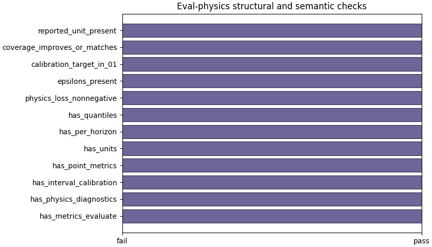
Plot the structural checks separately#
The boolean summary is not a replacement for interpretation, but it is an excellent first gate. It answers simple questions quickly:
did the file carry the expected sections?
were epsilons present?
was the calibration target plausible?
did calibrated coverage improve or at least not degrade?
were units reported?
When this panel fails, the user should slow down before trusting any performance story.
fig, ax = plt.subplots(
    figsize=(8.4, 4.8),
    constrained_layout=True,
)
plot_eval_physics_boolean_summary(
    record,
    ax=ax,
    title="Eval-physics structural and semantic checks",
    color=EVAL_PHYSICS_PALETTE["checks"],
    edgecolor="#1F2937",
    linewidth=0.8,
    alpha=0.9,
)
<Axes: title={'center': 'Eval-physics structural and semantic checks'}>
A practical decision rule#
For this artifact family, a useful reading rule is:
required sections exist,
forecast quality is acceptable for the problem,
epsilon values are finite and not obviously unstable,
calibration improves or preserves coverage,
the sharpness penalty remains explainable,
units are explicit enough for reporting.
This is not a mathematical certificate. It is a practical workflow decision rule to decide whether the run is mature enough to present, compare, or export further.
checks = summary["checks"]
must_pass = [
    "has_metrics_evaluate",
    "has_physics_diagnostics",
    "has_interval_calibration",
    "has_point_metrics",
    "has_units",
    "epsilons_present",
    "calibration_target_in_01",
    "reported_unit_present",
]
structurally_ready = all(bool(checks.get(name, False)) for name in must_pass)

coverage_ok = bool(checks.get("coverage_improves_or_matches", False))
phys_ok = (phys.get("epsilon_prior") is not None) and (phys.get("epsilon_cons") is not None)

print("\nDecision note")
if structurally_ready and coverage_ok and phys_ok:
    print(
        "This demo eval-physics artifact looks coherent enough "
        "for deeper scientific interpretation."
    )
elif structurally_ready:
    print(
        "The artifact is structurally valid, but its calibration or "
        "physics behavior deserves closer review before reporting."
    )
else:
    print(
        "This artifact should be reviewed carefully before you rely on it."
    )
Decision note
This demo eval-physics artifact looks coherent enough for deeper scientific interpretation.
Total running time of the script: (0 minutes 1.628 seconds)