Inspect a scaling_kwargs.json configuration

This lesson explains how to inspect one of the most important configuration artifacts in the GeoPrior workflow: scaling_kwargs.json.

Why this file matters

A Stage-1 / Stage-2 workflow can look healthy on the surface while still being inconsistent underneath. Many hard-to-diagnose problems come from configuration mismatches rather than from the neural model itself. Typical examples include:

• coordinates normalized in one step but interpreted as raw values later,

• a groundwater channel index that no longer matches the dynamic feature order,

• a forcing term Q interpreted with the wrong unit convention,

• bounds that are too wide, too narrow, or inconsistent with the chosen physics setup,

• a prior schedule that is much stronger or weaker than expected.

The goal of this lesson is therefore not only to display the configuration, but to teach how to read it and decide whether it is safe to proceed to training, diagnostics, or transfer.

What this lesson teaches

We will go step by step:

1. build a realistic scaling_kwargs artifact,

2. load it through the inspection layer,

3. summarize the most important decisions,

4. inspect coordinate conventions,

5. inspect feature-channel identities,

6. inspect affine SI maps,

7. inspect schedule and regularization scalars,

8. inspect bounds and boolean switches,

9. finish with a compact inspection bundle.

This page is written as a reading guide. After each view, we explain what the plot means, what is usually important, and what would count as a warning sign in a real workflow.

from __future__ import annotations

from pathlib import Path
from pprint import pprint
import tempfile

import matplotlib.pyplot as plt
import pandas as pd

from geoprior.utils.inspect import (
    generate_scaling_kwargs,
    inspect_scaling_kwargs,
    load_scaling_kwargs,
    plot_scaling_kwargs_affine_maps,
    plot_scaling_kwargs_boolean_summary,
    plot_scaling_kwargs_bounds,
    plot_scaling_kwargs_coord_ranges,
    plot_scaling_kwargs_feature_group_sizes,
    plot_scaling_kwargs_schedule_scalars,
    scaling_kwargs_affine_frame,
    scaling_kwargs_bounds_frame,
    scaling_kwargs_coord_frame,
    scaling_kwargs_feature_channels_frame,
    scaling_kwargs_schedule_frame,
    summarize_scaling_kwargs,
)

Create a realistic demo artifact

In documentation lessons we usually do not want to rerun the full GeoPrior pipeline just to obtain one artifact. The inspection layer is therefore designed to generate a realistic, stable demonstration file.

Here we intentionally make a few configuration choices slightly more explicit than the bare default so the lesson becomes easier to read:

• subs_scale_si = 1e-3 illustrates a common case where subsidence values are stored in millimetres and converted to metres,

• coords_normalized = True makes the coordinate range plot useful,

• a non-trivial MV-prior schedule makes the schedule section teachable.

None of this is meant to be the only correct setup. The point is to create a representative artifact that we can inspect like a real file.

workdir = Path(tempfile.mkdtemp(prefix="gp_sg_scaling_"))
json_path = workdir / "demo_scaling_kwargs.json"

_ = generate_scaling_kwargs(
    json_path,
    overrides={
        "subs_scale_si": 1e-3,
        "subs_bias_si": 0.0,
        "head_scale_si": 1.0,
        "H_scale_si": 1.0,
        "coords_normalized": True,
        "coord_ranges": {"t": 7.0, "x": 44447.0, "y": 39275.0},
        "Q_kind": "per_volume",
        "mv_weight": 0.005,
        "mv_delay_epochs": 2,
        "mv_warmup_epochs": 4,
        "track_aux_metrics": True,
    },
)

print("Written artifact:")
print(f" - {json_path}")

Written artifact:
 - /tmp/gp_sg_scaling_0vkb4vk3/demo_scaling_kwargs.json

Load the artifact through the inspection layer

The loader wraps the JSON inside a small artifact record so the rest of the inspection utilities can treat it consistently.

In a real workflow, this is the same pattern you would use on a file exported by Stage-1 or Stage-2.

record = load_scaling_kwargs(json_path)
payload = record.payload

SCALING_COLORS = {
    "primary": "#4f46e5",
    "secondary": "#0f766e",
    "accent": "#d97706",
    "rose": "#db2777",
    "ink": "#0f172a",
    "muted": "#64748b",
    "grid": "#cbd5e1",
    "face": "#f8fafc",
    "pass": "#16a34a",
    "fail": "#dc2626",
}


def _style_axes(ax: plt.Axes, *, facecolor: str = SCALING_COLORS["face"]) -> None:
    ax.set_facecolor(facecolor)
    ax.set_axisbelow(True)
    ax.grid(True, color=SCALING_COLORS["grid"], alpha=0.45, linewidth=0.8)
    for side in ("top", "right"):
        ax.spines[side].set_visible(False)
    for side in ("left", "bottom"):
        ax.spines[side].set_color("#94a3b8")
        ax.spines[side].set_linewidth(0.9)
    ax.tick_params(colors=SCALING_COLORS["ink"], labelsize=9)
    if ax.get_title():
        ax.set_title(ax.get_title(), fontsize=11, fontweight="bold", color=SCALING_COLORS["ink"], pad=12)
    if ax.get_xlabel():
        ax.set_xlabel(ax.get_xlabel(), fontsize=9.5, color=SCALING_COLORS["muted"])
    if ax.get_ylabel():
        ax.set_ylabel(ax.get_ylabel(), fontsize=9.5, color=SCALING_COLORS["muted"])


def _style_bars(ax: plt.Axes, colors: list[str], *, edgecolor: str = SCALING_COLORS["ink"], linewidth: float = 1.1, alpha: float = 0.95) -> None:
    for idx, patch in enumerate(ax.patches):
        patch.set_facecolor(colors[idx % len(colors)])
        patch.set_edgecolor(edgecolor)
        patch.set_linewidth(linewidth)
        patch.set_alpha(alpha)


def _style_boolean_bars(ax: plt.Axes) -> None:
    for patch in ax.patches:
        value = patch.get_width() if patch.get_width() else patch.get_height()
        color = SCALING_COLORS["pass"] if value >= 0.5 else SCALING_COLORS["fail"]
        patch.set_facecolor(color)
        patch.set_edgecolor(SCALING_COLORS["ink"])
        patch.set_linewidth(1.1)
        patch.set_alpha(0.95)


print("Artifact kind:", record.kind)
print("Artifact path:", record.path)

Artifact kind: scaling_kwargs
Artifact path: /tmp/gp_sg_scaling_0vkb4vk3/demo_scaling_kwargs.json

Read the high-level summary first

Before looking at any plot, it is often best to ask a compact question:

What kind of configuration is this?

The summary is useful because it answers the first inspection questions quickly:

• Are coordinates normalized?

• Are coordinates raw degrees or projected metres?

• What is the GWL convention?

• Is head reconstruction enabled?

• What is the forcing interpretation?

• How many dynamic, future, and static channels are expected?

• Does the file actually carry a bounds section?

This summary is usually the first thing to read before going deeper.

summary = summarize_scaling_kwargs(payload)
pprint(summary)

{'Q_kind': 'per_volume',
 'affine_maps': {'H_bias_si': 0.0,
                 'H_scale_si': 1.0,
                 'head_bias_si': 0.0,
                 'head_scale_si': 1.0,
                 'subs_bias_si': 0.0,
                 'subs_scale_si': 0.001},
 'coord_mode': 'degrees',
 'coord_order': ['t', 'x', 'y'],
 'coord_ranges': {'t': 7.0, 'x': 44447.0, 'y': 39275.0},
 'coords_in_degrees': False,
 'coords_normalized': True,
 'dynamic_features': 5,
 'future_features': 1,
 'gwl_kind': 'depth_bgs',
 'gwl_sign': 'down_positive',
 'has_bounds': True,
 'has_gwl_z_meta': True,
 'mv_prior_mode': 'calibrate',
 'mv_schedule_unit': 'epoch',
 'n_bounds': 14,
 'static_features': 12,
 'time_units': 'year',
 'use_head_proxy': True}

A first interpretation of the summary

When I inspect a file like this, I mentally check a few items in order:

1. Coordinate convention If coords_normalized is True, later derivative calculations must be interpreted together with coord_ranges. A user should never read a normalized coordinate tensor without also knowing those ranges.

2. Groundwater convention gwl_kind and gwl_sign tell us how the data entered the model. This matters because a physically correct model can still look wrong if depth, head, or sign conventions are mixed.

3. Feature counts The counts for dynamic, future, and static groups define the shape of several Stage-2 tensors. If these counts drift from the actual data order, the model may still run but learn from the wrong channels.

4. Bounds presence has_bounds is a fast health check. If the workflow expects soft or hard physical bounds and this is False, that is already a warning.

In other words, the summary is not the final diagnosis. It is the quickest way to decide where deeper inspection is needed.

Inspect coordinate metadata as a table

The coordinate table is the right place to verify how time and space are represented, not only whether they are normalized.

Things worth checking here:

• coord_order should match the convention used by your model and derivative code. In GeoPrior this is commonly t, x, y.

• coord_src_epsg and coord_target_epsg should make sense for the city and projection strategy.

• time_units should match how you think about rates and closures later in the physics terms.

• the ranges t/x/y should be plausible in magnitude.

A suspicious pattern would be something like:

• normalized coordinates with missing ranges,

• metre-like x/y values but coords_in_degrees=True, or

• tiny/zero ranges that would later explode derivative scaling.

coord_frame = scaling_kwargs_coord_frame(payload)
print(coord_frame.to_string(index=False))

     section              name        value
  coord_meta        coord_mode      degrees
  coord_meta       coord_order      t, x, y
  coord_meta    coord_src_epsg         4326
  coord_meta coord_target_epsg        32649
  coord_meta   coord_epsg_used        32649
  coord_meta        time_units         year
coord_ranges                 t     7.000000
coord_ranges                 x 44447.000000
coord_ranges                 y 39275.000000

Plot 1: coordinate ranges

This is the first plot I would show a user because it answers one of the most important practical questions:

If coordinates are normalized, what physical span does each axis represent?

How to read this plot:

• t is the time span represented by the normalized time coordinate.

• x and y are the spatial spans represented by normalized space.

• if x and y are very different, the domain is anisotropic and that can affect the intuitive scale of spatial derivatives.

What is important here is not whether the bars are large or small in an absolute sense, but whether they are plausible for the intended study area and time window.

fig, ax = plt.subplots(figsize=(7.2, 3.8))
plot_scaling_kwargs_coord_ranges(
    payload,
    ax=ax,
    title="Coordinate ranges carried by the scaling config",
)
_style_axes(ax, facecolor="#f8fafc")
_style_bars(ax, [SCALING_COLORS["primary"], SCALING_COLORS["secondary"], SCALING_COLORS["accent"]])
plt.show()

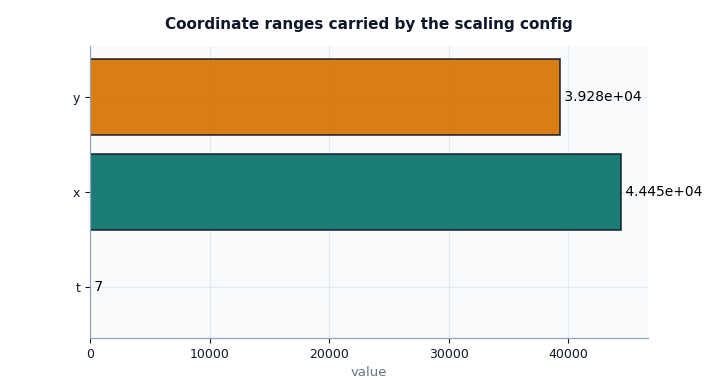
Interpret the coordinate plot

In this demo artifact, the spatial ranges are much larger than the time range. That is expected because t is expressed in years while x and y are metre spans.

The important lesson is this:

• a normalized coordinate tensor alone is not enough to interpret PDE derivatives,

• the scaling config must preserve the corresponding physical ranges,

• if these ranges are wrong, residual magnitudes and closures can become misleading even if the model code itself is correct.

Inspect feature-group sizes and channel identity

The next question is structural:

Do the named channels still match the tensor layout expected by the model?

The group-size plot is simple, but it is very useful because many downstream files only store tensor shapes. This plot reconnects those shapes to human-readable channel groups.

fig, ax = plt.subplots(figsize=(7.2, 3.6))
plot_scaling_kwargs_feature_group_sizes(
    payload,
    ax=ax,
    title="Feature-group sizes declared in scaling_kwargs",
)
_style_axes(ax, facecolor="#fbfcff")
_style_bars(ax, [SCALING_COLORS["secondary"], SCALING_COLORS["accent"], SCALING_COLORS["primary"]])
plt.show()

feature_frame = scaling_kwargs_feature_channels_frame(payload)
print(feature_frame.to_string(index=False))

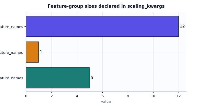
          group                  name               value
 feature_counts dynamic_feature_names                   5
 feature_counts  future_feature_names                   1
 feature_counts  static_feature_names                  12
channel_indices         gwl_dyn_index            0.000000
channel_indices        subs_dyn_index            1.000000
channel_indices   z_surf_static_index           11.000000
  channel_names          gwl_dyn_name GWL_depth_bgs_m__si
  channel_names               gwl_col GWL_depth_bgs_m__si
  channel_names        gwl_target_col          head_m__si
  channel_names        subs_model_col  subsidence_cum__si
  channel_names            z_surf_col        z_surf_m__si

How to read the feature-channel section

This section is critical when debugging Stage-2 handshakes.

Focus on three levels:

1. Group counts These tell you how many channels belong to each tensor family.

2. Channel indices gwl_dyn_index and subs_dyn_index tell the model where to find important dynamic signals inside the dynamic tensor.

3. Channel names These names help you verify that the semantic meaning still matches the index.

A strong warning sign is when the index and the name no longer agree, for example:

• gwl_dyn_index = 0 but the first dynamic feature name is not the groundwater channel,

• z_surf_static_index points to a non-topographic feature,

• the counts implied by the lists do not match the tensor shapes used later in Stage-2.

When users say “the model runs but the physics feels wrong”, this is one of the first places I would inspect.

Inspect affine SI maps

The affine maps explain how model-space values are converted back into SI-like physical quantities. This is a small section, but it is central for interpretability.

In this lesson we intentionally set subs_scale_si = 1e-3 so the conversion is visible in the plot.

affine_frame = scaling_kwargs_affine_frame(payload)
print(affine_frame.to_string(index=False))

fig, ax = plt.subplots(figsize=(8.0, 4.2))
plot_scaling_kwargs_affine_maps(
    payload,
    ax=ax,
    title="Affine SI maps for subsidence, head, and thickness",
)
_style_axes(ax, facecolor="#fffdf8")
_style_bars(ax, [SCALING_COLORS["accent"], SCALING_COLORS["rose"], SCALING_COLORS["secondary"], SCALING_COLORS["primary"], SCALING_COLORS["accent"], SCALING_COLORS["secondary"]])
plt.show()

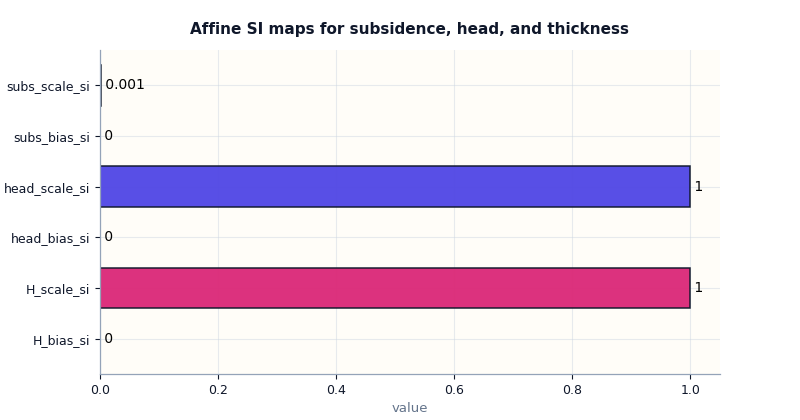
    parameter    value           unit
subs_scale_si 0.001000 m / model-unit
 subs_bias_si 0.000000              m
head_scale_si 1.000000 m / model-unit
 head_bias_si 0.000000              m
   H_scale_si 1.000000 m / model-unit
    H_bias_si 0.000000              m

What the affine-map plot tells us

A user should read this plot with one main question in mind:

Are these variables already in physical units, or do they still need a meaningful conversion?

In our demo:

• the subsidence scale is non-trivial, so a model-space subsidence value is converted into metres using a factor of 1e-3,

• the head and thickness maps are identity-like, which usually means those channels already entered the workflow in a physical unit that the model keeps directly.

This matters because evaluation metrics, plotted maps, and physics payloads can all look numerically sensible while still being off by a unit factor if these affine maps are misunderstood.

Inspect schedule and regularization scalars

The next section answers a different kind of question:

How strongly will the configuration regularize or gate parts of the training and physics behaviour?

This is where users should look when training is either too unstable, too weakly constrained, or unexpectedly slow to activate certain priors.

schedule_frame = scaling_kwargs_schedule_frame(payload)
print(schedule_frame.to_string(index=False))

fig, ax = plt.subplots(figsize=(8.4, 4.8))
plot_scaling_kwargs_schedule_scalars(
    payload,
    ax=ax,
    title="Schedule and runtime scalars carried by the config",
)
_style_axes(ax, facecolor="#f8fafc")
_style_bars(ax, [SCALING_COLORS["primary"], SCALING_COLORS["secondary"], SCALING_COLORS["accent"], SCALING_COLORS["rose"]])
plt.show()

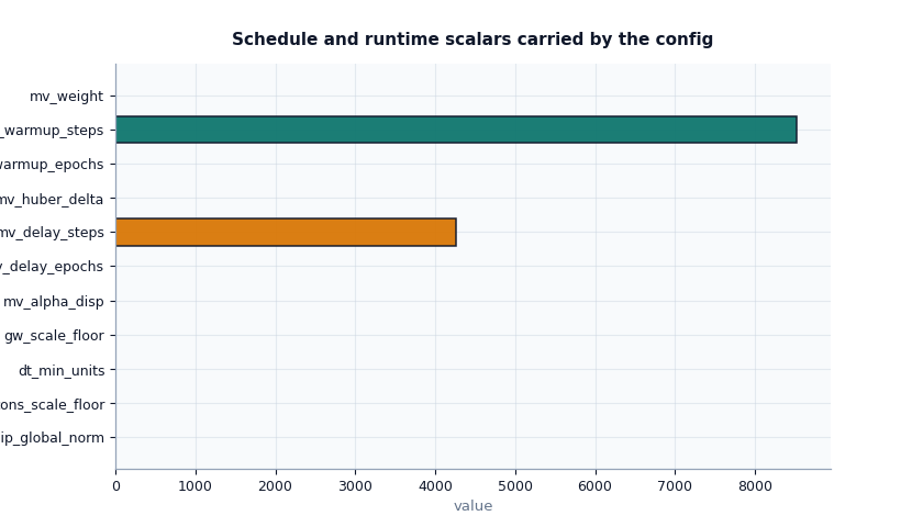
        section                 name         value
scalar_schedule     clip_global_norm      5.000000
scalar_schedule     cons_scale_floor      0.000000
scalar_schedule       gw_scale_floor      0.000000
scalar_schedule         dt_min_units      0.000001
scalar_schedule            mv_weight      0.005000
scalar_schedule        mv_alpha_disp      0.100000
scalar_schedule       mv_huber_delta      1.000000
scalar_schedule      mv_delay_epochs      2.000000
scalar_schedule     mv_warmup_epochs      4.000000
scalar_schedule       mv_delay_steps   4261.000000
scalar_schedule      mv_warmup_steps   8522.000000
          modes               Q_kind    per_volume
          modes        mv_prior_mode     calibrate
          modes       mv_prior_units        strict
          modes     mv_schedule_unit         epoch
          modes  cons_residual_units        second
          modes    gw_residual_units        second
          modes        drainage_mode        double
          modes scaling_error_policy         raise
          modes             gwl_kind     depth_bgs
          modes             gwl_sign down_positive

How to interpret the schedule section

A few values deserve special attention:

• clip_global_norm: tells you how aggressively gradients may be clipped. Too low can suppress learning; too high may allow unstable steps.

• cons_scale_floor and gw_scale_floor: protect residual scaling from collapsing toward zero.

• mv_weight: controls how strongly the MV prior contributes.

• mv_delay_* and mv_warmup_*: tell you when that prior starts to matter.

• Q_kind and mv_prior_mode: they are not scalar magnitudes, but they strongly affect the physical meaning of later residual terms.

In practice, if a user complains that a prior “never seems to kick in”, the first thing I would check is whether the delay and warmup schedule in this file matches the number of epochs or steps actually used in the run.

Inspect bounds carefully

Bounds deserve their own section because they define the admissible physical range for important latent quantities such as K, Ss, and tau.

Users often read a bounds plot too quickly. The most important idea is not simply “higher or lower”, but whether the bounds are:

• present,

• internally consistent,

• plausible for the intended geophysical setting,

• broad enough to allow learning,

• narrow enough to encode prior knowledge.

bounds_frame = scaling_kwargs_bounds_frame(payload)
print(bounds_frame.to_string(index=False))

fig, ax = plt.subplots(figsize=(8.8, 5.2))
plot_scaling_kwargs_bounds(
    payload,
    ax=ax,
    title="Configured physical and log-space bounds",
)
_style_axes(ax, facecolor="#fffdfa")
_style_bars(ax, [SCALING_COLORS["primary"], SCALING_COLORS["accent"], SCALING_COLORS["secondary"], SCALING_COLORS["rose"]])
ax.tick_params(axis="y", labelsize=8.5)
plt.show()

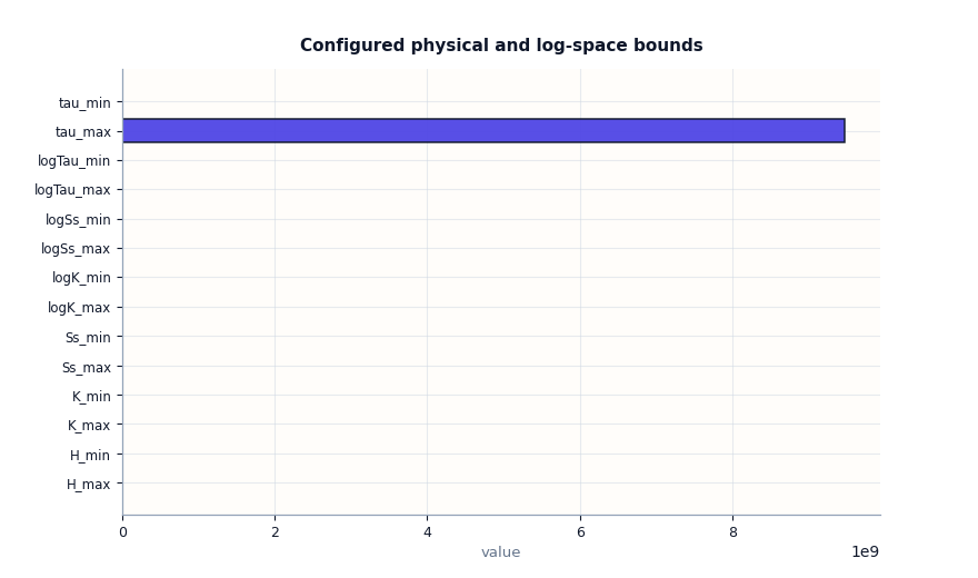
     bound             value
     H_min          0.100000
     H_max         30.000000
     K_min          0.000000
     K_max          0.000000
    Ss_min          0.000001
    Ss_max          0.001000
   tau_min     604800.000000
   tau_max 9467085600.000000
  logK_min        -27.631021
  logK_max        -16.118096
 logSs_min        -13.815511
 logSs_max         -6.907755
logTau_min         13.312653
logTau_max         22.971087

What is especially important in the bounds plot

There are two families of bounds here:

1. Linear-space bounds such as K_min / K_max and Ss_min / Ss_max.

2. Log-space bounds such as logK_min / logK_max and logSs_min / logSs_max.

Both are useful because many models operate internally in log space even when users think about the corresponding physical values in linear space.

A good lesson to remember is this: if the linear and log bounds do not describe the same intended range, later interpretation becomes confusing. Even when the code runs, the model may appear more or less constrained than the user expects.

Inspect boolean switches as workflow checks

Boolean flags are easy to underestimate. They often look small, but they switch important behaviours on or off.

This plot is particularly good for a final “sanity sweep” because it helps users catch configuration contradictions quickly.

fig, ax = plt.subplots(figsize=(8.2, 4.2))
plot_scaling_kwargs_boolean_summary(
    payload,
    ax=ax,
    title="Boolean switches worth checking before training",
)
_style_axes(ax, facecolor="#f8fafc")
_style_boolean_bars(ax)
plt.show()

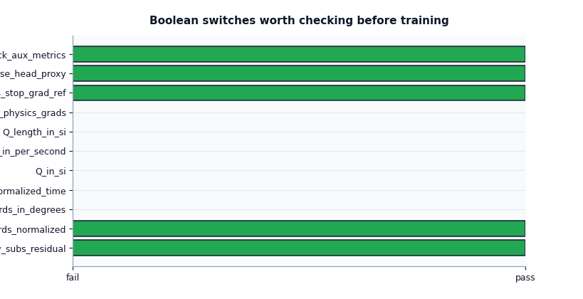
How to read the boolean summary

I usually read the boolean summary as a set of workflow questions:

• Are coordinates normalized?

• Are coordinates still in degrees?

• Is forcing interpreted with normalized time?

• Is the config claiming SI input for Q?

• Is head proxy reconstruction enabled?

• Are auxiliary metrics tracked?

The goal is not that every answer be True. The goal is that the answers are coherent together.

For example:

• coords_normalized=True is reasonable,

• but if coord_ranges were missing, that would be a problem,

• use_head_proxy=True is reasonable,

• but then the groundwater metadata should also explain how head is derived from depth and surface elevation.

Build a compact inspection bundle

After reading each section individually, it is convenient to build a compact bundle that gathers the main tables in one place.

In a real project, this is useful when you want to archive a quick review or pass a concise summary to a teammate.

bundle = inspect_scaling_kwargs(payload)

print("Inspection bundle keys:")
print(sorted(bundle))

print("\nCompact summary again:")
pprint(bundle["summary"])

Inspection bundle keys:
['affine', 'bounds', 'coords', 'features', 'schedule', 'summary']

Compact summary again:
{'Q_kind': 'per_volume',
 'affine_maps': {'H_bias_si': 0.0,
                 'H_scale_si': 1.0,
                 'head_bias_si': 0.0,
                 'head_scale_si': 1.0,
                 'subs_bias_si': 0.0,
                 'subs_scale_si': 0.001},
 'coord_mode': 'degrees',
 'coord_order': ['t', 'x', 'y'],
 'coord_ranges': {'t': 7.0, 'x': 44447.0, 'y': 39275.0},
 'coords_in_degrees': False,
 'coords_normalized': True,
 'dynamic_features': 5,
 'future_features': 1,
 'gwl_kind': 'depth_bgs',
 'gwl_sign': 'down_positive',
 'has_bounds': True,
 'has_gwl_z_meta': True,
 'mv_prior_mode': 'calibrate',
 'mv_schedule_unit': 'epoch',
 'n_bounds': 14,
 'static_features': 12,
 'time_units': 'year',
 'use_head_proxy': True}

Final decision checklist

Before moving on to Stage-2 training or downstream diagnostics, a user should be able to answer the following questions confidently:

• Do I understand whether coordinates are raw or normalized?

• Are the time and space ranges plausible?

• Do the named channels still agree with the declared indices?

• Are the SI affine maps sensible for the variables I will interpret?

• Does the prior and schedule configuration match my training plan?

• Are the physical bounds present and plausible?

• Are the boolean switches mutually coherent?

If the answer to one of these is “not sure”, this file should be fixed before trusting later metrics, physics diagnostics, or forecasts.

In a real workflow, simply replace json_path with the path to your own exported scaling_kwargs.json artifact and rerun the same lesson.