Build a stratified spatial sample table

This example teaches you how to use GeoPrior’s spatial-sampling build utility.

Unlike figure-generation pages, this lesson starts from a tabular workflow. The goal is to build a smaller table that still preserves:

• the broad spatial footprint,

• the balance across years,

• the balance across cities,

• and the balance across geological classes.

Why this matters

Large geospatial tables are often too heavy for quick prototyping, debugging, teaching, or compact downstream examples. A good spatial sample should be smaller, but it should not lose the main structure of what makes the dataset useful.

That is exactly what spatial-sampling is for.

Imports

We call the real production entrypoint from the project code. For the synthetic dataset itself, we reuse the robust spatial support helpers from geoprior.scripts.utils instead of generating ad hoc random coordinates by hand.

from __future__ import annotations

import tempfile
from pathlib import Path

import matplotlib.pyplot as plt
import numpy as np
import pandas as pd

from geoprior.cli.build_spatial_sampling import (
    build_spatial_sampling_main,
)
from geoprior.scripts.utils import (
    SpatialSupportSpec,
    make_spatial_field,
    make_spatial_scale,
    make_spatial_support,
)

Build two synthetic city supports

Each city support is created from SpatialSupportSpec. The parameters are commented deliberately so readers can see how the spatial cloud is controlled.

Important ideas:

• center_x and center_y place the city support.

• span_x and span_y control the city size.

• nx and ny control the mesh density before masking.

• jitter_x and jitter_y add small coordinate irregularity.

• footprint chooses the synthetic city shape.

• keep_frac optionally thins the support after masking.

• seed keeps the support reproducible.

ns_spec = SpatialSupportSpec(
    city="Nansha",
    center_x=113.52,
    center_y=22.74,
    span_x=0.17,
    span_y=0.11,
    nx=62,
    ny=48,
    jitter_x=0.0014,
    jitter_y=0.0012,
    footprint="nansha_like",
    keep_frac=0.84,
    seed=7,
)

zh_spec = SpatialSupportSpec(
    city="Zhongshan",
    center_x=113.38,
    center_y=22.53,
    span_x=0.19,
    span_y=0.13,
    nx=64,
    ny=50,
    jitter_x=0.0015,
    jitter_y=0.0012,
    footprint="zhongshan_like",
    keep_frac=0.82,
    seed=19,
)

ns_support = make_spatial_support(ns_spec)
zh_support = make_spatial_support(zh_spec)

print("Synthetic support sizes")
print(f" - Nansha   : {ns_support.sample_idx.size:,} points")
print(f" - Zhongshan: {zh_support.sample_idx.size:,} points")

Synthetic support sizes
 - Nansha   : 1,244 points
 - Zhongshan: 1,225 points

Convert the spatial supports into a panel-like dataset

spatial-sampling works on ordinary tables, so we now turn the supports into a richer DataFrame with:

• spatial coordinates,

• a time column,

• categorical stratification columns,

• and one continuous target-like field.

We keep the geometry synthetic, but the structure realistic enough to teach why stratified sampling matters.

rng = np.random.default_rng(42)

years = [2021, 2022, 2023, 2024]
frames: list[pd.DataFrame] = []

for support, amp0, drift_x, drift_y in [
    (ns_support, 7.4, 0.11, 0.08),
    (zh_support, 8.1, 0.07, 0.10),
]:
    base_mean = make_spatial_field(
        support,
        amplitude=amp0,
        drift_x=drift_x,
        drift_y=drift_y,
        phase=0.20,
        hotspot_weight=0.92,
        secondary_weight=0.56,
        ridge_weight=0.18,
        wave_weight=0.14,
        local_weight=0.05,
    )

    for year in years:
        step = year - years[0]
        scale = make_spatial_scale(
            support,
            base=0.35,
            x_weight=0.10,
            hotspot_weight=0.07,
            step_weight=0.03,
            step=step,
        )

        year_boost = 0.75 * step
        mean = base_mean + year_boost
        noise = rng.normal(0.0, scale * 0.55)

        frame = support.to_frame().rename(
            columns={
                "coord_x": "longitude",
                "coord_y": "latitude",
            }
        )
        frame["year"] = int(year)

        # A categorical class that varies across the city footprint.
        frame["lithology_class"] = np.where(
            frame["y_norm"] > 0.62,
            "Clay",
            np.where(frame["x_norm"] > 0.57, "Fill", "Sand"),
        )

        # A second categorical field can be useful later for other
        # builders, even though this lesson only stratifies on the
        # lithology class.
        frame["development_zone"] = np.where(
            frame["x_norm"] + frame["y_norm"] > 1.08,
            "Urban core",
            "Expansion belt",
        )

        frame["rainfall_mm"] = (
            1320
            + 85 * step
            + 45 * frame["y_norm"]
            + rng.normal(0.0, 14.0, len(frame))
        )
        frame["subsidence_mm"] = mean + noise

        frames.append(frame)

full_df = pd.concat(frames, ignore_index=True)

print("")
print("Synthetic input table")
print(full_df.head(8).to_string(index=False))

Synthetic input table
 sample_idx  longitude  latitude  x_norm  y_norm   city  year lithology_class development_zone  rainfall_mm  subsidence_mm
          0   113.4994   22.6596  0.4389  0.1443 Nansha  2021            Sand   Expansion belt    1341.1237         0.0440
          1   113.5322   22.6589  0.5339  0.1412 Nansha  2021            Sand   Expansion belt    1327.3070        -0.4666
          2   113.4671   22.6647  0.3456  0.1670 Nansha  2021            Sand   Expansion belt    1321.7446         0.6510
          3   113.4837   22.6639  0.3936  0.1635 Nansha  2021            Sand   Expansion belt    1302.0500         0.4470
          4   113.4869   22.6646  0.4029  0.1664 Nansha  2021            Sand   Expansion belt    1325.0875        -0.2093
          5   113.4958   22.6624  0.4286  0.1566 Nansha  2021            Sand   Expansion belt    1305.2141        -0.2172
          6   113.5035   22.6645  0.4509  0.1660 Nansha  2021            Sand   Expansion belt    1341.0144         0.0566
          7   113.5207   22.6627  0.5004  0.1581 Nansha  2021            Sand   Expansion belt    1348.3502        -0.1689

Write one input file per city

The shared build-reader utilities accept one or many input files, so the lesson demonstrates the multi-file workflow directly.

tmp_dir = Path(
    tempfile.mkdtemp(prefix="gp_sg_spatial_sampling_")
)

ns_csv = tmp_dir / "nansha_spatial_panel.csv"
zh_csv = tmp_dir / "zhongshan_spatial_panel.csv"

full_df.loc[full_df["city"] == "Nansha"].to_csv(
    ns_csv,
    index=False,
)
full_df.loc[full_df["city"] == "Zhongshan"].to_csv(
    zh_csv,
    index=False,
)

print("")
print("Input files")
print(" -", ns_csv.name)
print(" -", zh_csv.name)

Input files
 - nansha_spatial_panel.csv
 - zhongshan_spatial_panel.csv

Run the real spatial-sampling builder

We ask the command to:

• read both city files,

• build spatial bins on longitude and latitude,

• preserve balance across city, year, and lithology class,

• and write a compact CSV sample.

We use relative mode here because it is especially helpful when some stratification groups are smaller than others.

out_csv = tmp_dir / "spatial_sampling_gallery.csv"

build_spatial_sampling_main(
    [
        str(ns_csv),
        str(zh_csv),
        "--sample-size",
        "0.18",
        "--stratify-by",
        "city",
        "year",
        "lithology_class",
        "--spatial-cols",
        "longitude",
        "latitude",
        "--spatial-bins",
        "8",
        "7",
        "--method",
        "relative",
        "--min-relative-ratio",
        "0.03",
        "--random-state",
        "42",
        "--output",
        str(out_csv),
        "--verbose",
        "1",
    ]
)

Creating spat. bins: 2:   0%|                          | 0/2 [00:00<?, ?it/s]
Creating spat. bins: 2: 100%|#################| 2/2 [00:00<00:00, 459.27it/s]
Data grouped into 272 stratified bins.

Sampling 1,777 records:   0%|                        | 0/272 [00:00<?, ?it/s]
Sampling 1,777 records:  77%|#########2  | 209/272 [00:00<00:00, 2088.89it/s]
Sampling 1,777 records: 100%|############| 272/272 [00:00<00:00, 2059.04it/s]

Sampling completed: 1,768 records selected.
[OK] loaded 9,876 row(s) and wrote 1,768 sampled row(s) to /tmp/gp_sg_spatial_sampling_rzvaznsh/spatial_sampling_gallery.csv

Inspect the written sample

The builder writes one output table. We read it back and inspect its structure exactly as a user would do after running the command.

sampled_df = pd.read_csv(out_csv)

print("")
print("Written file")
print(" -", out_csv.name)

print("")
print("Sampled table")
print(sampled_df.head(10).to_string(index=False))

Written file
 - spatial_sampling_gallery.csv

Sampled table
 sample_idx  longitude  latitude  x_norm  y_norm   city  year lithology_class development_zone  rainfall_mm  subsidence_mm
       1153   113.4532   22.8029  0.3055  0.7782 Nansha  2021            Clay       Urban core    1352.4550         1.1780
        875   113.4418   22.7682  0.2725  0.6248 Nansha  2021            Clay   Expansion belt    1358.9308         2.0623
        914   113.4549   22.7707  0.3104  0.6358 Nansha  2021            Clay   Expansion belt    1358.0966         3.4760
       1154   113.4618   22.8034  0.3303  0.7805 Nansha  2021            Clay       Urban core    1346.1023         1.6080
        981   113.4547   22.7805  0.3096  0.6791 Nansha  2021            Clay   Expansion belt    1353.8418         2.7037
       1119   113.4560   22.7975  0.3135  0.7543 Nansha  2021            Clay   Expansion belt    1360.6693         1.5934
       1123   113.4854   22.7992  0.3985  0.7617 Nansha  2021            Clay       Urban core    1348.8491         2.1964
        954   113.4935   22.7751  0.4218  0.6553 Nansha  2021            Clay   Expansion belt    1346.4783         4.2377
        881   113.4765   22.7674  0.3729  0.6212 Nansha  2021            Clay   Expansion belt    1350.6567         4.3708
       1055   113.4741   22.7897  0.3659  0.7199 Nansha  2021            Clay       Urban core    1348.1107         3.3676

Compare the full table and the sampled table

A good lesson should not stop at “the command ran”. We also want to show why the output is useful.

The tables below compare how the sample keeps the main structure of the original dataset.

city_year_full = (
    full_df.groupby(["city", "year"]).size().rename("n_full")
)
city_year_sample = (
    sampled_df.groupby(["city", "year"]).size().rename("n_sample")
)
city_year_cmp = pd.concat(
    [city_year_full, city_year_sample],
    axis=1,
).fillna(0)
city_year_cmp["sample_rate"] = (
    city_year_cmp["n_sample"] / city_year_cmp["n_full"]
)
city_year_cmp = city_year_cmp.reset_index()

lith_full = (
    full_df.groupby(["city", "lithology_class"])
    .size()
    .rename("n_full")
)
lith_sample = (
    sampled_df.groupby(["city", "lithology_class"])
    .size()
    .rename("n_sample")
)
lith_cmp = pd.concat(
    [lith_full, lith_sample],
    axis=1,
).fillna(0)
lith_cmp["sample_rate"] = (
    lith_cmp["n_sample"] / lith_cmp["n_full"]
)
lith_cmp = lith_cmp.reset_index()

print("")
print("City-year comparison")
print(city_year_cmp.to_string(index=False))

print("")
print("City-lithology comparison")
print(lith_cmp.to_string(index=False))

City-year comparison
     city  year  n_full  n_sample  sample_rate
   Nansha  2021    1244       224       0.1801
   Nansha  2022    1244       224       0.1801
   Nansha  2023    1244       224       0.1801
   Nansha  2024    1244       224       0.1801
Zhongshan  2021    1225       218       0.1780
Zhongshan  2022    1225       218       0.1780
Zhongshan  2023    1225       218       0.1780
Zhongshan  2024    1225       218       0.1780

City-lithology comparison
     city lithology_class  n_full  n_sample  sample_rate
   Nansha            Clay    1360       244       0.1794
   Nansha            Fill    1464       264       0.1803
   Nansha            Sand    2152       388       0.1803
Zhongshan            Clay    1052       184       0.1749
Zhongshan            Fill    1608       292       0.1816
Zhongshan            Sand    2240       396       0.1768

Build one compact visual preview

Top row:

original footprint and sampled footprint.

Bottom row:

city-year sample rates and lithology sample rates.

This visual preview is just for the lesson page. The production command itself only writes the sampled table.

fig, axes = plt.subplots(
    2,
    2,
    figsize=(10.2, 8.2),
    constrained_layout=True,
)

city_colors = {
    "Nansha": "tab:blue",
    "Zhongshan": "tab:red",
}

# Original footprint.
ax = axes[0, 0]
for city in ["Nansha", "Zhongshan"]:
    sub = full_df.loc[full_df["city"] == city]
    ax.scatter(
        sub["longitude"],
        sub["latitude"],
        s=6,
        alpha=0.35,
        label=city,
        color=city_colors[city],
    )
ax.set_title("Original synthetic table")
ax.set_xlabel("Longitude")
ax.set_ylabel("Latitude")
ax.legend(loc="best")
ax.grid(True, linestyle=":", alpha=0.4)

# Sampled footprint.
ax = axes[0, 1]
for city in ["Nansha", "Zhongshan"]:
    sub = sampled_df.loc[sampled_df["city"] == city]
    ax.scatter(
        sub["longitude"],
        sub["latitude"],
        s=10,
        alpha=0.70,
        label=city,
        color=city_colors[city],
    )
ax.set_title("Sampled output table")
ax.set_xlabel("Longitude")
ax.set_ylabel("Latitude")
ax.legend(loc="best")
ax.grid(True, linestyle=":", alpha=0.4)

# City-year sample rates.
ax = axes[1, 0]
labels = [
    f"{row.city}\n{int(row.year)}"
    for row in city_year_cmp.itertuples(index=False)
]
ax.bar(
    np.arange(len(city_year_cmp)),
    city_year_cmp["sample_rate"].to_numpy(),
)
ax.set_title("Sample rate by city and year")
ax.set_ylabel("Sample rate")
ax.set_xticks(np.arange(len(city_year_cmp)))
ax.set_xticklabels(labels, rotation=35, ha="right")
ax.grid(True, axis="y", linestyle=":", alpha=0.4)

# City-lithology sample rates.
ax = axes[1, 1]
labels = [
    f"{row.city}\n{row.lithology_class}"
    for row in lith_cmp.itertuples(index=False)
]
ax.bar(
    np.arange(len(lith_cmp)),
    lith_cmp["sample_rate"].to_numpy(),
)
ax.set_title("Sample rate by city and lithology")
ax.set_ylabel("Sample rate")
ax.set_xticks(np.arange(len(lith_cmp)))
ax.set_xticklabels(labels, rotation=35, ha="right")
ax.grid(True, axis="y", linestyle=":", alpha=0.4)

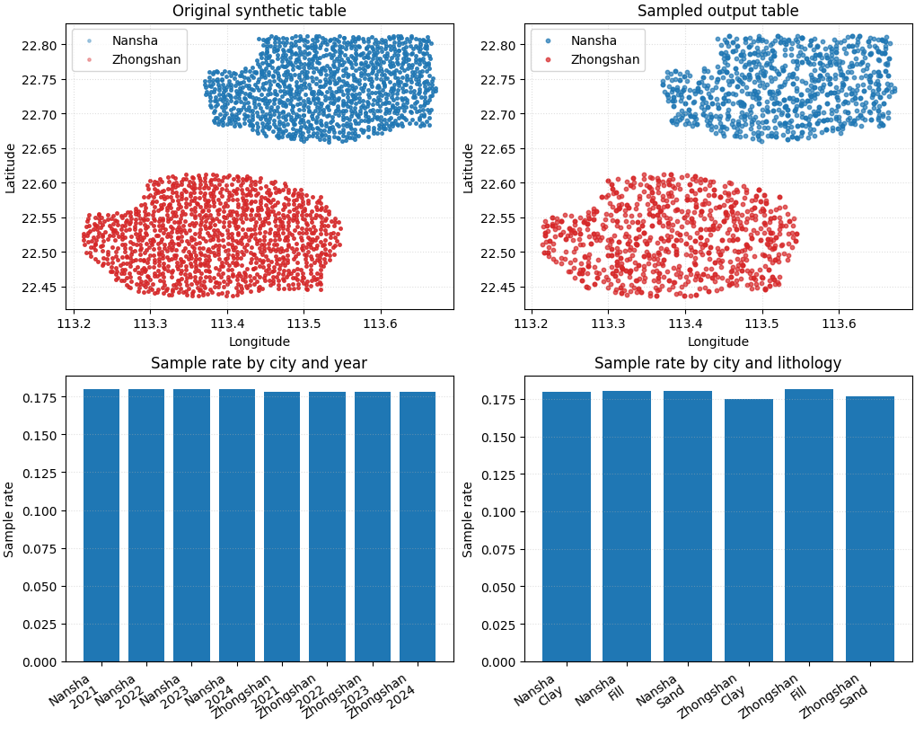
How to read this output

The goal is not to make every sample rate identical.

Instead, the goal is to make the smaller table remain representative:

• both city footprints should still be visible,

• each year should still appear,

• each lithology class should still be present,

• and the sampled table should remain easy to save and reuse.

This is why spatial-sampling is a strong table builder for:

• demos,

• debugging,

• quick benchmarking,

• tutorial pages,

• and lightweight downstream examples.

Command-line usage

The same workflow can be run directly from the command line.

Family entry point:

geoprior-build spatial-sampling \
    nansha_spatial_panel.csv \
    zhongshan_spatial_panel.csv \
    --sample-size 0.18 \
    --stratify-by city year lithology_class \
    --spatial-cols longitude latitude \
    --spatial-bins 8 7 \
    --method relative \
    --min-relative-ratio 0.03 \
    --random-state 42 \
    --output spatial_sampling_gallery.csv

Root entry point:

geoprior build spatial-sampling \
    nansha_spatial_panel.csv \
    zhongshan_spatial_panel.csv \
    --sample-size 0.18 \
    --stratify-by city year lithology_class \
    --spatial-cols longitude latitude \
    --spatial-bins 8 7 \
    --method relative \
    --min-relative-ratio 0.03 \
    --random-state 42 \
    --output spatial_sampling_gallery.csv

Because the shared reader accepts multiple table types, the same command family can also be used with:

• one file or many files,

• CSV / TSV / Parquet / Excel / JSON / Feather / Pickle,

• and Excel sheet selectors such as input.xlsx::Sheet1.