Diagnostics#
This gallery focuses on workflow diagnostics, split credibility, training behavior, tuning interpretation, and physics-consistency checks in GeoPrior.
Unlike the forecasting gallery, which explains how forecast outputs are built and read, and unlike the uncertainty gallery, which explains how probabilistic forecasts are calibrated and interpreted, the pages collected here are organized around a different practical question:
How should a user check whether the workflow itself is behaving sensibly before trusting later forecast and physics results?
The emphasis is therefore on diagnostic credibility. These examples show how GeoPrior turns preprocessing logic, training histories, tuning artifacts, and physics summaries into readable workflow diagnostics such as:
group-validity masks,
holdout split designs,
training-curve summaries,
hyperparameter tuning summaries,
bridge diagnostics from training to physics inspection.
In other words, this gallery is about checking the workflow: not training the final model itself, and not yet producing the final forecast or physics figures.
What this gallery teaches#
Most pages in this section follow the same broad pattern:
create a compact synthetic workflow artifact,
call the real GeoPrior helper or mimic its output contract,
inspect the returned tables, splits, curves, or summaries,
explain how to read and interpret the diagnostic result.
Even when a page prints small tables or summaries, the main goal remains the same: to explain the diagnostic artifact and its interpretation.
Module guide#
Module |
Main output |
Purpose |
|---|---|---|
|
Group-validity masks |
Compute which spatial groups are valid for training and which remain usable only for forecasting, then filter the raw table accordingly. |
|
Holdout split design |
Compare random and spatial-block train/validation/test group splits and explain why spatial-block holdout is often more credible for geospatial forecasting. |
|
Stage-1 data-validity and split diagnostics |
Check which spatial groups are valid for training or only for forecasting, filter the raw table accordingly, and compare random versus spatial-block holdout credibility. |
|
Training-history diagnostics |
Read Stage-2 loss curves, physics-loss components, validation behavior, and warmup / scaling controls. |
|
Tuning-summary diagnostics |
Inspect Stage-3 hyperparameter search results, top trials, search progression, and parameter-versus-score structure. |
|
Physics bridge diagnostics |
Connect training diagnostics to later physics inspection using timescale consistency, field distributions, residual summaries, and payload-based diagnostics. |
Reading path#
A useful way to move through this gallery is to follow the logic of a complete workflow check:
begin by checking whether the data groups are valid and whether the holdout split is credible,
inspect Stage-2 training behavior,
inspect Stage-3 tuning behavior,
finish with the bridge from optimization diagnostics to physics diagnostics.
That is why the examples are grouped by workflow-diagnostic purpose rather than only by utility or plotting function.
Gallery organization#
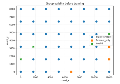
Stage-1 validity checks#
These examples are the best place to start when you want to know whether the data are even usable for the intended workflow.
They focus on questions such as:
which groups contain all required training years,
which groups contain enough years only for forecasting,
how much of the dataset survives early filtering.
The main page in this group is:
holdout_group_masks.py
Holdout-split credibility#
These examples focus on the design of the train/validation/test split.
They are most useful when you want to inspect:
whether train, validation, and test groups are disjoint,
how random splitting differs from spatial-block splitting,
whether the chosen split strategy is too optimistic for a spatial forecasting problem.
The main page in this group is:
spatial_block_holdout.py
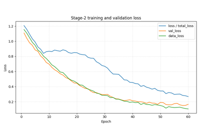
Stage-2 training diagnostics#
These examples focus on optimization behavior during model fitting.
They are especially useful when you want to inspect:
whether training and validation loss behave sensibly,
whether the supervised and physics losses are balanced,
whether epsilon-style residual diagnostics improve,
whether warmup or scaling controls are shaping the run.
The main page in this group is:
plot_stage2_training_curves.py
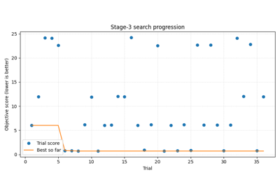
Stage-3 tuning diagnostics#
These examples focus on hyperparameter search behavior.
They are most useful when you want to inspect:
whether the search kept improving,
whether the best trial is clearly better than the rest,
which hyperparameters seem associated with better performance,
whether the winning trial is also stable and practical.
The main page in this group is:
plot_stage3_tuning_summary.py
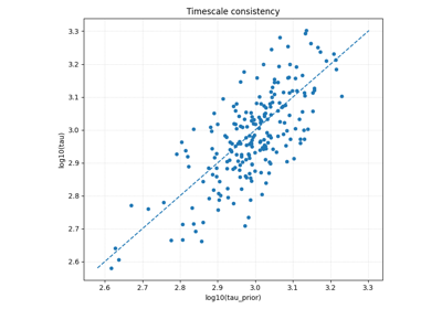
Physics diagnostic bridge#
These examples focus on the transition from workflow diagnostics to physics interpretation.
They are particularly useful when you want to inspect:
whether learned and closure-implied timescales agree,
whether physics fields have plausible distributions,
whether residual-like quantities are centered and stable,
how to move from training diagnostics to flat payload-based physics analysis.
The main page in this group is:
physics_diagnostic_bridge.py
Why this separation matters#
This gallery deliberately keeps four concerns distinct:
Stage-1 data and split checks,
Stage-2 optimization diagnostics,
Stage-3 tuning diagnostics,
bridge diagnostics into physics inspection.
That separation makes the workflow easier to understand. It also helps users distinguish between:
helpers that validate which groups are usable,
helpers that define the credibility of the holdout split,
diagnostic summaries that explain how training and tuning behaved,
and bridge artifacts that prepare later physics inspection.
Notes#
These examples are intentionally compact and lesson-oriented.
The pages in this section are diagnostics-first: they may print tables, split summaries, or metric summaries, but their main purpose is to explain how the workflow should be checked before later forecasts or physics figures are trusted.
A useful rule of thumb is:
forecasting/explains how forecast outputs are built, read, and evaluated,uncertainty/explains calibration, reliability, and event-risk interpretation,diagnostics/explains workflow validity, training behavior, tuning behavior, and the bridge into physics diagnostics,tables_and_summaries/builds reusable analysis artifacts.
A practical reading sequence is:
first validate the groups,
then inspect the holdout strategy,
then inspect Stage-2 training curves,
then inspect Stage-3 tuning summaries,
then move to the physics diagnostic bridge before reading later model-inspection or figure-generation pages.
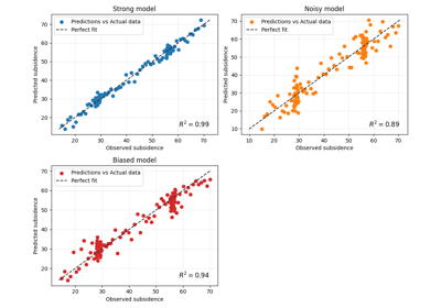
Physics diagnostics bridge: from evaluate_physics to payload inspection
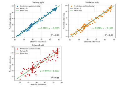
Compare independent regression pairs with plot_r2_in
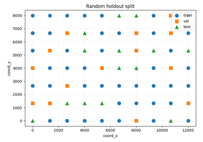
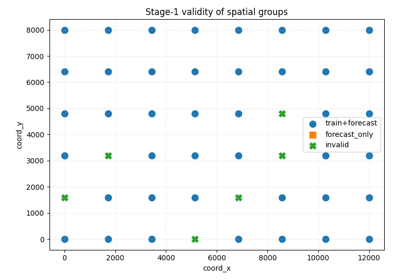
Stage-1 data checks with group masks and holdout splitting
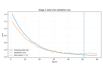
Stage-2 training curves and physics-aware learning dynamics