From raw model outputs to forecast tables with format_and_forecast

This lesson teaches one of the most important utilities in the forecasting workflow: geoprior.utils.forecast_utils.format_and_forecast().

Why this page matters

Most plotting pages in the forecasting gallery start from already formatted forecast tables such as:

• df_eval: evaluation rows with predictions and actuals,

• df_future: future rows with predictions only.

But a real model does not produce those tables directly.

Instead, the model produces raw arrays such as:

• y_pred["subs_pred"] with shape (B, H, Q, O) in quantile mode,

• y_true[...] with shape (B, H, O),

• optional coords with shape (B, H, 3).

The job of format_and_forecast is to convert those raw outputs into clean, long-format DataFrames that downstream tools can inspect, plot, and evaluate.

What the real function does

The utility takes raw prediction dictionaries, optional truth arrays, optional coordinates, and temporal configuration, then returns:

• df_eval: predictions + actuals for the evaluation side,

• df_future: predictions for the future horizon.

It supports quantile mode, point mode, optional spatial coordinates, evaluation export control, cumulative or absolute-cumulative transformations, optional calibration, and optional calls to evaluate_forecast.

The resulting DataFrames carry a standard structure centered on sample_idx, forecast_step, coord_t, optional coord_x/coord_y, prediction columns such as subsidence_q10 / subsidence_q50 / subsidence_q90 or subsidence_pred, and an actual column for the evaluation side. That is exactly why the later forecasting pages can read these outputs directly.

What this lesson teaches

We will:

1. build synthetic spatial forecast data that mimics a real city grid,

2. create raw y_pred and y_true arrays in the same shape a probabilistic model would return,

3. call the real format_and_forecast utility,

4. inspect the resulting evaluation and future forecast tables,

5. show how eval_export changes what is written on the evaluation side,

6. show how value_mode changes rate forecasts into cumulative and absolute cumulative forecasts,

7. finish by sending the resulting tables into a real plotting helper.

The example is fully synthetic so the page is executable during the documentation build.

Imports

We use the real utility that the forecasting workflow relies on.

import numpy as np
import pandas as pd

from geoprior.plot import plot_eval_future
from geoprior.utils.forecast_utils import (
    evaluate_forecast,
    format_and_forecast,
)

Step 1 - Build a compact synthetic spatial layout

We mimic a small city-like spatial grid.

Each spatial location becomes one “sample” from the perspective of the forecast formatting utility. The model will later return H-step forecasts for every one of these samples.

rng = np.random.default_rng(42)

nx = 7
ny = 5
xv = np.linspace(0.0, 12_000.0, nx)
yv = np.linspace(0.0, 8_000.0, ny)

X, Y = np.meshgrid(xv, yv)
x_flat = X.ravel()
y_flat = Y.ravel()

B = x_flat.size          # number of spatial samples
H = 3                    # forecast horizon
Q = 3                    # q10, q50, q90
O = 1                    # one subsidence target

quantiles = [0.1, 0.5, 0.9]
future_years = np.array([2023, 2024, 2025], dtype=int)
train_end_year = 2022

print("Number of samples (B):", B)
print("Forecast horizon (H):", H)
print("Quantiles (Q):", quantiles)

Number of samples (B): 35
Forecast horizon (H): 3
Quantiles (Q): [0.1, 0.5, 0.9]

Step 2 - Build synthetic raw coordinates in model layout

format_and_forecast expects optional coordinates shaped like (B, H, 3) with columns typically interpreted as:

• t

• x

• y

Importantly, the function uses x/y for spatial coordinates, while the time column is overwritten by the temporal configuration when we provide train_end_time and future_time_grid. So the time values inside coords are not the main source of truth here.

coords = np.zeros((B, H, 3), dtype=float)

for i in range(B):
    for h in range(H):
        coords[i, h, 0] = h + 1         # placeholder t-like slot
        coords[i, h, 1] = x_flat[i]     # x
        coords[i, h, 2] = y_flat[i]     # y

print("coords shape:", coords.shape)

coords shape: (35, 3, 3)

Step 3 - Build synthetic raw model outputs

We now create arrays that mimic a probabilistic subsidence model.

Target contract:

• y_pred["subs_pred"] in quantile mode: shape (B, H, Q, O)

• y_true["subsidence"]: shape (B, H, O)

The synthetic field is designed so that:

• one main hotspot exists,

• a secondary ridge is present,

• the response strengthens through time,

• the predictive interval widens with horizon.

xn = (x_flat - x_flat.min()) / (x_flat.max() - x_flat.min())
yn = (y_flat - y_flat.min()) / (y_flat.max() - y_flat.min())

hotspot = np.exp(
    -(
        ((xn - 0.72) ** 2) / 0.022
        + ((yn - 0.34) ** 2) / 0.030
    )
)
ridge = 0.55 * np.exp(
    -(
        ((xn - 0.26) ** 2) / 0.030
        + ((yn - 0.70) ** 2) / 0.060
    )
)
gradient = 0.48 * xn + 0.22 * (1.0 - yn)

# raw true values: (B, H, O)
y_true_subs = np.zeros((B, H, O), dtype=float)

# raw predicted quantiles: (B, H, Q, O)
y_pred_subs = np.zeros((B, H, Q, O), dtype=float)

for h in range(H):
    year_scale = [1.00, 1.18, 1.42][h]

    median = (
        1.9
        + 1.4 * gradient
        + 2.0 * hotspot
        + 0.95 * ridge
    ) * year_scale

    width = (
        0.28
        + 0.07 * xn
        + 0.05 * hotspot
        + 0.05 * (h + 1)
    )

    q10 = median - width
    q50 = median
    q90 = median + width

    # truth stays close to q50 but is not identical
    actual = median + rng.normal(0.0, 0.14, size=B)

    y_true_subs[:, h, 0] = actual
    y_pred_subs[:, h, 0, 0] = q10
    y_pred_subs[:, h, 1, 0] = q50
    y_pred_subs[:, h, 2, 0] = q90

y_pred = {"subs_pred": y_pred_subs}
y_true = {"subsidence": y_true_subs}

print("y_pred['subs_pred'] shape:", y_pred["subs_pred"].shape)
print("y_true['subsidence'] shape:", y_true["subsidence"].shape)

y_pred['subs_pred'] shape: (35, 3, 3, 1)
y_true['subsidence'] shape: (35, 3, 1)

Step 4 - Call the real format_and_forecast utility

This is the main lesson step.

Important settings:

• quantiles=[0.1, 0.5, 0.9]: quantile mode, so the function emits q10/q50/q90 columns;

• train_end_time=2022: anchors the evaluation-side time reconstruction;

• future_time_grid=[2023, 2024, 2025]: explicit future horizon labels;

• eval_export="all": export all evaluation horizons rather than only the final one;

• value_mode="rate": treat each step as an incremental forecast, not yet cumulative.

In the real implementation, eval_forecast_step defaults to the last horizon if not provided, and eval_export="all" promotes the multi-horizon evaluation DataFrame when it is available.

df_eval, df_future = format_and_forecast(
    y_pred=y_pred,
    y_true=y_true,
    coords=coords,
    quantiles=quantiles,
    target_name="subsidence",
    train_end_time=train_end_year,
    future_time_grid=future_years,
    eval_export="all",
    value_mode="rate",
    city_name="SyntheticCity",
    model_name="GeoPrior-demo",
    dataset_name="synthetic-spatial-grid",
    verbose=0,
)

print("df_eval shape:", df_eval.shape)
print("df_future shape:", df_future.shape)

print("")
print("df_eval head")
print(df_eval.head(10).to_string(index=False))

print("")
print("df_future head")
print(df_future.head(10).to_string(index=False))

df_eval shape: (105, 9)
df_future shape: (105, 8)

df_eval head
 sample_idx  forecast_step   coord_t  subsidence_actual  subsidence_q10  subsidence_q50  subsidence_q90   coord_x  coord_y
          0              1 2020.0000             2.2507          1.8780          2.2080          2.5380    0.0000   0.0000
          0              2 2021.0000             2.7635          2.2255          2.6055          2.9855    0.0000   0.0000
          0              3 2022.0000             2.9568          2.7054          3.1354          3.5654    0.0000   0.0000
          1              1 2020.0000             2.1745          1.9784          2.3201          2.6618 2000.0000   0.0000
          1              2 2021.0000             2.7218          2.3461          2.7377          3.1294 2000.0000   0.0000
          1              3 2022.0000             3.1359          2.8529          3.2946          3.7362 2000.0000   0.0000
          2              1 2020.0000             2.5372          2.0788          2.4322          2.7855 4000.0000   0.0000
          2              2 2021.0000             2.7523          2.4666          2.8700          3.2733 4000.0000   0.0000
          2              3 2022.0000             3.3250          3.0003          3.4537          3.9070 4000.0000   0.0000
          3              1 2020.0000             2.6804          2.1836          2.5487          2.9138 6000.0000   0.0000

df_future head
 sample_idx  forecast_step  subsidence_q10  subsidence_q50  subsidence_q90  coord_t   coord_x  coord_y
          0              1          1.8780          2.2080          2.5380     2023    0.0000   0.0000
          0              2          2.2255          2.6055          2.9855     2024    0.0000   0.0000
          0              3          2.7054          3.1354          3.5654     2025    0.0000   0.0000
          1              1          1.9784          2.3201          2.6618     2023 2000.0000   0.0000
          1              2          2.3461          2.7377          3.1294     2024 2000.0000   0.0000
          1              3          2.8529          3.2946          3.7362     2025 2000.0000   0.0000
          2              1          2.0788          2.4322          2.7855     2023 4000.0000   0.0000
          2              2          2.4666          2.8700          3.2733     2024 4000.0000   0.0000
          2              3          3.0003          3.4537          3.9070     2025 4000.0000   0.0000
          3              1          2.1836          2.5487          2.9138     2023 6000.0000   0.0000

Step 5 - Understand the two returned DataFrames

df_eval and df_future are the central products of this function.

On the evaluation side we expect:

• sample_idx

• forecast_step

• coord_t

• coord_x, coord_y

• quantile columns

• subsidence_actual

On the future side we expect the same prediction structure, but no actual column because those years are beyond the observed data window. The implementation explicitly drops the actual column from the future DataFrame.

print("")
print("df_eval columns")
print(df_eval.columns.tolist())

print("")
print("df_future columns")
print(df_future.columns.tolist())

df_eval columns
['sample_idx', 'forecast_step', 'coord_t', 'subsidence_actual', 'subsidence_q10', 'subsidence_q50', 'subsidence_q90', 'coord_x', 'coord_y']

df_future columns
['sample_idx', 'forecast_step', 'subsidence_q10', 'subsidence_q50', 'subsidence_q90', 'coord_t', 'coord_x', 'coord_y']

A compact year / horizon summary helps explain the table layout.

eval_summary = (
    df_eval.groupby(["coord_t", "forecast_step"])
    .agg(
        n_rows=("sample_idx", "size"),
        mean_q50=("subsidence_q50", "mean"),
        mean_actual=("subsidence_actual", "mean"),
    )
    .reset_index()
)

future_summary = (
    df_future.groupby(["coord_t", "forecast_step"])
    .agg(
        n_rows=("sample_idx", "size"),
        mean_q10=("subsidence_q10", "mean"),
        mean_q50=("subsidence_q50", "mean"),
        mean_q90=("subsidence_q90", "mean"),
    )
    .reset_index()
)

print("")
print("Evaluation summary")
print(eval_summary.to_string(index=False))

print("")
print("Future summary")
print(future_summary.to_string(index=False))

Evaluation summary
  coord_t  forecast_step  n_rows  mean_q50  mean_actual
2020.0000              1      35    2.5469       2.5530
2021.0000              2      35    3.0054       3.0153
2022.0000              3      35    3.6166       3.5820

Future summary
 coord_t  forecast_step  n_rows  mean_q10  mean_q50  mean_q90
    2023              1      35    2.1792    2.5469    2.9147
    2024              2      35    2.5876    3.0054    3.4231
    2025              3      35    3.1489    3.6166    4.0844

What these summaries mean

The evaluation DataFrame here is multi-horizon because we used eval_export="all".

That means the evaluation side now contains one row per:

• sample

• forecast step

rather than only the final evaluation step.

This is one of the most important things to understand about the utility: the returned table can represent either a single-step evaluation view or the full multi-horizon evaluation view depending on the export control.

Step 6 - Compare eval_export="all" versus eval_export="last"

The easiest way to understand eval_export is to run the function twice and compare the outputs.

df_eval_last, df_future_last = format_and_forecast(
    y_pred=y_pred,
    y_true=y_true,
    coords=coords,
    quantiles=quantiles,
    target_name="subsidence",
    train_end_time=train_end_year,
    future_time_grid=future_years,
    eval_export="last",
    value_mode="rate",
    verbose=0,
)

print("Rows with eval_export='all': ", len(df_eval))
print("Rows with eval_export='last':", len(df_eval_last))

print("")
print("Single-step evaluation head")
print(df_eval_last.head(8).to_string(index=False))

Rows with eval_export='all':  105
Rows with eval_export='last': 35

Single-step evaluation head
 sample_idx  forecast_step  subsidence_q10  subsidence_q50  subsidence_q90  subsidence_actual   coord_t    coord_x   coord_y
          0              3          2.7054          3.1354          3.5654             2.9568 2022.0000     0.0000    0.0000
          1              3          2.8529          3.2946          3.7362             3.1359 2022.0000  2000.0000    0.0000
          2              3          3.0003          3.4537          3.9070             3.3250 2022.0000  4000.0000    0.0000
          3              3          3.1541          3.6192          4.0843             3.6888 2022.0000  6000.0000    0.0000
          4              3          3.3469          3.8244          4.3020             3.8444 2022.0000  8000.0000    0.0000
          5              3          3.4752          3.9642          4.4531             4.0608 2022.0000 10000.0000    0.0000
          6              3          3.5913          4.0913          4.5913             4.0315 2022.0000 12000.0000    0.0000
          7              3          2.5987          3.0287          3.4587             3.0509 2022.0000     0.0000 2000.0000

Interpretation

Use:

• eval_export="all" when you want full multi-horizon evaluation analysis or horizon-wise metrics;

• eval_export="last" when you want the compact, single-step evaluation table that mirrors the original backward-compatible behavior.

Step 7 - Demonstrate cumulative and absolute cumulative modes

Another important lesson in this utility is that it can reinterpret the horizon values as:

• rates,

• relative cumulative values,

• absolute cumulative values.

In the real implementation:

• "cumulative" applies a cumulative sum by sample over forecast_step,

• "absolute_cumulative" does the same and then adds a baseline value or mapping.

baseline_map = {
    int(i): 12.0 + 0.5 * np.sin(i / 4.0)
    for i in range(B)
}

df_eval_abs, df_future_abs = format_and_forecast(
    y_pred=y_pred,
    y_true=y_true,
    coords=coords,
    quantiles=quantiles,
    target_name="subsidence",
    train_end_time=train_end_year,
    future_time_grid=future_years,
    eval_export="all",
    value_mode="absolute_cumulative",
    absolute_baseline=baseline_map,
    verbose=0,
)

cum_summary = (
    df_future_abs.groupby("coord_t")
    .agg(
        mean_q50=("subsidence_q50", "mean"),
        mean_q90=("subsidence_q90", "mean"),
    )
    .reset_index()
)

print("")
print("Absolute cumulative future summary")
print(cum_summary.to_string(index=False))

Absolute cumulative future summary
 coord_t  mean_q50  mean_q90
    2023   14.6437   15.0114
    2024   17.6491   18.4345
    2025   21.2657   22.5189

Why this matters

The same raw model output can support different downstream stories.

• In rate mode, each step is interpreted as a per-step increment.

• In cumulative mode, the horizon becomes an accumulated path.

• In absolute cumulative mode, the path is shifted to an absolute reference level.

That distinction is crucial in geohazard forecasting because users may want either:

• incremental annual change,

• relative cumulative change since the start of the horizon,

• or absolute cumulative state referenced to the end of training.

Step 8 - Run automatic forecast evaluation

format_and_forecast can optionally trigger the evaluation helper, but for a lesson page it is often clearer to call evaluate_forecast explicitly afterward.

The evaluator is designed around the same DataFrame contract and computes deterministic metrics plus coverage and sharpness in quantile mode. It can also compute per-horizon metrics.

metrics = evaluate_forecast(
    df_eval,
    target_name="subsidence",
    per_horizon=True,
    quantile_interval=(0.1, 0.9),
    verbose=0,
)

print("")
print("Evaluation metrics")
print(metrics)

Evaluation metrics
{'2020.0': {'overall_mae': 0.09316328621789392, 'overall_mse': 0.013194267953305815, 'overall_rmse': 0.11486630469073955, 'overall_r2': 0.9313993409609541, 'coverage80': 1.0, 'sharpness80': 0.7354701962484429, 'per_horizon_mae': {1: 0.09316328621789392}, 'per_horizon_mse': {1: 0.013194267953305815}, 'per_horizon_rmse': {1: 0.11486630469073955}, 'per_horizon_r2': {1: 0.9313993409609541}}, '2021.0': {'overall_mae': 0.0858458413840222, 'overall_mse': 0.010454926931111198, 'overall_rmse': 0.10224933706929937, 'overall_r2': 0.9581072028908791, 'coverage80': 1.0, 'sharpness80': 0.8354701962484429, 'per_horizon_mae': {2: 0.0858458413840222}, 'per_horizon_mse': {2: 0.010454926931111198}, 'per_horizon_rmse': {2: 0.10224933706929937}, 'per_horizon_r2': {2: 0.9581072028908791}}, '2022.0': {'overall_mae': 0.09146411233712559, 'overall_mse': 0.011824409621731901, 'overall_rmse': 0.10874010125860607, 'overall_r2': 0.9670756101050856, 'coverage80': 1.0, 'sharpness80': 0.9354701962484429, 'per_horizon_mae': {3: 0.09146411233712559}, 'per_horizon_mse': {3: 0.011824409621731901}, 'per_horizon_rmse': {3: 0.10874010125860607}, 'per_horizon_r2': {3: 0.9670756101050856}}, '__overall__': {'overall_mae': 0.09015774664634722, 'overall_mse': 0.011824534835382972, 'overall_rmse': 0.10874067700443552, 'overall_r2': 0.9733720334822351, 'coverage80': 1.0, 'sharpness80': 0.835470196248443, 'per_horizon_mae': {1: 0.09316328621789392, 2: 0.0858458413840222, 3: 0.09146411233712559}, 'per_horizon_mse': {1: 0.013194267953305815, 2: 0.010454926931111198, 3: 0.011824409621731901}, 'per_horizon_rmse': {1: 0.11486630469073955, 2: 0.10224933706929937, 3: 0.10874010125860607}, 'per_horizon_r2': {1: 0.9313993409609541, 2: 0.9581072028908791, 3: 0.9670756101050856}}}

How to read these metrics

The main things to inspect are:

• overall_mae / overall_mse / overall_r2: central forecast accuracy,

• coverage80: how often the actual value falls inside the q10-q90 interval,

• sharpness80: average interval width,

• per_horizon_*: whether accuracy degrades across the horizon.

This is why format_and_forecast is such a key bridge utility: once the tables exist, both plotting and evaluation become simple.

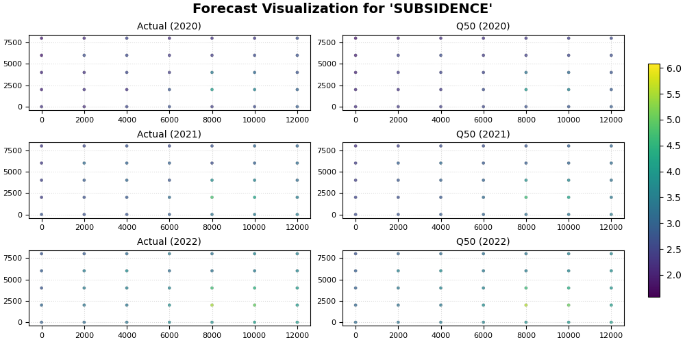
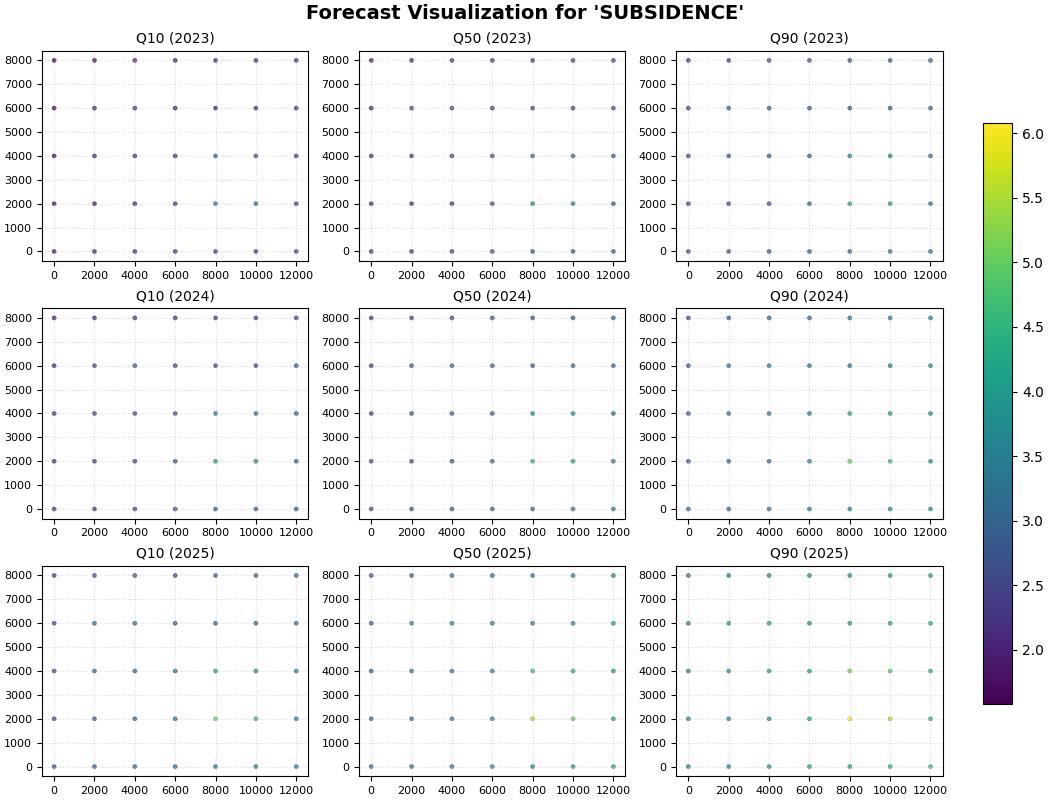
Step 9 - Send the formatted tables into a real plotting function

To close the lesson, we connect this utility page to the rest of the forecasting gallery.

The tables returned here can be passed directly into plot_eval_future for a holdout-versus-future comparison.

plot_eval_future(
    df_eval=df_eval,
    df_future=df_future,
    target_name="subsidence",
    quantiles=quantiles,
    spatial_cols=("coord_x", "coord_y"),
    time_col="coord_t",
    eval_years=[2020, 2021, 2022],
    future_years=[2023, 2024, 2025],
    eval_view_quantiles=[0.5],
    future_view_quantiles=[0.1, 0.5, 0.9],
    cbar="uniform",
    axis_off=False,
    show_grid=True,
    grid_props={"linestyle": ":", "alpha": 0.45},
    figsize_eval=(10.0, 5.0),
    figsize_future=(10.5, 8.0),
    show=True,
    verbose=0,
)

• 
• 

Final lesson takeaway

format_and_forecast is the utility that turns raw model arrays into the canonical long-format forecast tables used across the forecasting workflow.

Once you understand this function, the rest of the forecasting gallery becomes much easier to read because you know exactly where the tables come from and why they have the columns they do.