
Note
Go to the end to download the full example code.
Summarize hotspot point clouds into tidy group tables#
This example teaches you how to use GeoPrior’s
summarize-hotspots utility.
Unlike the plotting scripts, this command is a table builder. It starts from a hotspot point cloud CSV and converts it into a tidy summary grouped by city, year, and hotspot kind.
Why this matters#
A hotspot map or point cloud is useful for visual inspection, but it is not yet the compact artifact that downstream analysis usually needs.
This builder converts hotspot points into a grouped table with:
hotspot counts,
min/mean/max hotspot subsidence values,
min/mean/max hotspot anomaly values,
optional baseline summaries,
optional threshold summaries.
That makes it a strong lesson page for the
tables_and_summaries section.
Imports#
We call the real production entrypoint from the project code. Then we read the generated CSV back in and build one compact teaching preview.
from __future__ import annotations

import tempfile
from pathlib import Path

import matplotlib.pyplot as plt
import numpy as np
import pandas as pd

from geoprior.scripts.summarize_hotspots import (
    summarize_hotspots,
    summarize_hotspots_main,
)
Build a compact synthetic hotspot point cloud#
The real script expects a hotspot CSV produced by the spatial forecast workflow, with fields such as:
city
year
kind
value
metric_value
and optionally:
baseline_value
threshold
For the lesson, we create two cities, three years, and two hotspot kinds. That is enough to show how the builder groups the point cloud into one summary row per (city, year, kind).
rng = np.random.default_rng(11)

rows: list[dict[str, object]] = []

for city in ["Nansha", "Zhongshan"]:
    city_shift = 0.0 if city == "Nansha" else 6.0

    for year in [2025, 2027, 2030]:
        year_shift = {2025: 0.0, 2027: 3.5, 2030: 8.0}[year]

        for kind in ["q50", "q90"]:
            kind_shift = 0.0 if kind == "q50" else 5.0

            n_hot = 12 if kind == "q50" else 8
            if city == "Zhongshan":
                n_hot += 3

            baseline_mean = 36.0 + city_shift
            threshold = 11.0 + 0.7 * year_shift + 0.4 * kind_shift

            for i in range(n_hot):
                coord_x = 100 + rng.normal(0.0, 18.0)
                coord_y = 200 + rng.normal(0.0, 14.0)

                metric_value = max(
                    0.1,
                    threshold
                    + rng.normal(2.8 + 0.2 * year_shift, 1.3),
                )

                baseline_value = max(
                    0.1,
                    baseline_mean + rng.normal(0.0, 2.2),
                )

                value = baseline_value + metric_value

                rows.append(
                    {
                        "city": city,
                        "panel": "future_hotspots",
                        "kind": kind,
                        "year": year,
                        "coord_x": float(coord_x),
                        "coord_y": float(coord_y),
                        "value": float(value),
                        "hotspot_mode": "delta_abs",
                        "hotspot_quantile": 0.90,
                        "metric_value": float(metric_value),
                        "baseline_value": float(baseline_value),
                        "threshold": float(threshold),
                    }
                )

hotspots_df = pd.DataFrame(rows)

print("Hotspot point-cloud preview")
print(hotspots_df.head(10).to_string(index=False))
Hotspot point-cloud preview
  city           panel kind  year  coord_x  coord_y   value hotspot_mode  hotspot_quantile  metric_value  baseline_value  threshold
Nansha future_hotspots  q50  2025 100.6155 219.0365 50.2695    delta_abs            0.9000       15.3921         34.8773    11.0000
Nansha future_hotspots  q50  2025  94.6365 192.6166 50.4173    delta_abs            0.9000       14.5406         35.8767    11.0000
Nansha future_hotspots  q50  2025 113.4439 174.1375 51.6244    delta_abs            0.9000       15.8365         35.7878    11.0000
Nansha future_hotspots  q50  2025 112.2468 198.0881 50.3260    delta_abs            0.9000       13.3072         37.0188    11.0000
Nansha future_hotspots  q50  2025 114.8412 197.1646 51.1099    delta_abs            0.9000       13.6014         37.5085    11.0000
Nansha future_hotspots  q50  2025  84.3339 178.7986 48.8382    delta_abs            0.9000       14.3135         34.5248    11.0000
Nansha future_hotspots  q50  2025  65.4339 188.6032 46.5671    delta_abs            0.9000       13.1921         33.3750    11.0000
Nansha future_hotspots  q50  2025  73.1357 200.5129 50.4535    delta_abs            0.9000       14.9664         35.4871    11.0000
Nansha future_hotspots  q50  2025  86.6153 205.3899 50.0724    delta_abs            0.9000       14.7324         35.3400    11.0000
Nansha future_hotspots  q50  2025 109.8040 214.6003 47.7412    delta_abs            0.9000       13.5310         34.2103    11.0000
Write the synthetic hotspot CSV#
The production command consumes a point-cloud CSV, so we follow the same workflow here.
tmp_dir = Path(
    tempfile.mkdtemp(prefix="gp_sg_hotspots_summary_")
)
hotspot_csv = tmp_dir / "fig6_hotspot_points.synthetic.csv"

hotspots_df.to_csv(hotspot_csv, index=False)

print("")
print(f"Input hotspot CSV written to: {hotspot_csv}")
Input hotspot CSV written to: /tmp/gp_sg_hotspots_summary_ocgu5__9/fig6_hotspot_points.synthetic.csv
Run the real summarizer#
We ask the production command to build the grouped summary CSV.
out_csv = tmp_dir / "fig6_hotspot_summary.csv"

summarize_hotspots_main(
    [
        "--hotspot-csv",
        str(hotspot_csv),
        "--out",
        str(out_csv),
        "--quiet",
        "false",
    ],
    prog="summarize-hotspots",
)
     city  year kind  n_hotspots  value_min  value_mean  value_max  metric_min  metric_mean  metric_max  baseline_min  baseline_max  baseline_mean  threshold_min  threshold_max
   Nansha  2025  q50     12.0000    46.5671     49.4705    51.6244     11.5458      14.1823     15.8365       33.1739       37.5085        35.2882        11.0000        11.0000
   Nansha  2025  q90      8.0000    50.1120     52.9304    57.3783     13.5020      16.3759     17.6013       33.0696       39.9406        36.5545        13.0000        13.0000
   Nansha  2027  q50     12.0000    49.1654     52.7279    55.9298     15.3097      17.1285     19.5806       32.0881       38.6542        35.5994        13.4500        13.4500
   Nansha  2027  q90      8.0000    48.9804     55.0306    58.4324     16.1703      19.0887     21.7183       32.8101       40.4233        35.9420        15.4500        15.4500
   Nansha  2030  q50     12.0000    53.7489     56.8669    59.5841     19.0182      20.3903     22.2338       34.1392       38.1938        36.4766        16.6000        16.6000
   Nansha  2030  q90      8.0000    54.0185     57.7708    63.7386     21.5822      22.7645     24.0733       30.9021       39.6653        35.0063        18.6000        18.6000
Zhongshan  2025  q50     15.0000    53.3934     57.1740    61.2156     11.7490      14.0620     15.8060       39.2505       46.4539        43.1120        11.0000        11.0000
Zhongshan  2025  q90     11.0000    53.8707     59.0115    66.2886     12.1832      15.5184     16.4947       40.2590       49.9718        43.4931        13.0000        13.0000
Zhongshan  2027  q50     15.0000    55.8386     58.9779    61.2734     13.3199      17.2894     19.2169       36.8076       44.2371        41.6885        13.4500        13.4500
Zhongshan  2027  q90     11.0000    57.1924     60.3965    65.2812     17.0242      19.0553     20.8428       38.2264       46.0037        41.3412        15.4500        15.4500
Zhongshan  2030  q50     15.0000    57.8785     62.6666    67.5113     18.5462      21.1885     23.1967       37.4222       45.5846        41.4780        16.6000        16.6000
Zhongshan  2030  q90     11.0000    61.8799     65.4382    69.0123     21.8191      23.3426     24.6560       39.0328       44.3724        42.0956        18.6000        18.6000

[OK] summary -> /tmp/gp_sg_hotspots_summary_ocgu5__9/fig6_hotspot_summary.csv
Read the generated summary table#
The output has one row per (city, year, kind) group.
summary = pd.read_csv(out_csv)

print("")
print("Written file")
print(" -", out_csv.name)

print("")
print("Grouped summary table")
print(summary.to_string(index=False))
Written file
 - fig6_hotspot_summary.csv

Grouped summary table
     city  year kind  n_hotspots  value_min  value_mean  value_max  metric_min  metric_mean  metric_max  baseline_min  baseline_max  baseline_mean  threshold_min  threshold_max
   Nansha  2025  q50     12.0000    46.5671     49.4705    51.6244     11.5458      14.1823     15.8365       33.1739       37.5085        35.2882        11.0000        11.0000
   Nansha  2025  q90      8.0000    50.1120     52.9304    57.3783     13.5020      16.3759     17.6013       33.0696       39.9406        36.5545        13.0000        13.0000
   Nansha  2027  q50     12.0000    49.1654     52.7279    55.9298     15.3097      17.1285     19.5806       32.0881       38.6542        35.5994        13.4500        13.4500
   Nansha  2027  q90      8.0000    48.9804     55.0306    58.4324     16.1703      19.0887     21.7183       32.8101       40.4233        35.9420        15.4500        15.4500
   Nansha  2030  q50     12.0000    53.7489     56.8669    59.5841     19.0182      20.3903     22.2338       34.1392       38.1938        36.4766        16.6000        16.6000
   Nansha  2030  q90      8.0000    54.0185     57.7708    63.7386     21.5822      22.7645     24.0733       30.9021       39.6653        35.0063        18.6000        18.6000
Zhongshan  2025  q50     15.0000    53.3934     57.1740    61.2156     11.7490      14.0620     15.8060       39.2505       46.4539        43.1120        11.0000        11.0000
Zhongshan  2025  q90     11.0000    53.8707     59.0115    66.2886     12.1832      15.5184     16.4947       40.2590       49.9718        43.4931        13.0000        13.0000
Zhongshan  2027  q50     15.0000    55.8386     58.9779    61.2734     13.3199      17.2894     19.2169       36.8076       44.2371        41.6885        13.4500        13.4500
Zhongshan  2027  q90     11.0000    57.1924     60.3965    65.2812     17.0242      19.0553     20.8428       38.2264       46.0037        41.3412        15.4500        15.4500
Zhongshan  2030  q50     15.0000    57.8785     62.6666    67.5113     18.5462      21.1885     23.1967       37.4222       45.5846        41.4780        16.6000        16.6000
Zhongshan  2030  q90     11.0000    61.8799     65.4382    69.0123     21.8191      23.3426     24.6560       39.0328       44.3724        42.0956        18.6000        18.6000
Compare with the direct in-memory API#
The script also exposes the core grouping function directly. This is useful for tests and notebook workflows.
summary_api = summarize_hotspots(hotspots_df)

print("")
print("Direct API result matches CSV output:")
print(summary_api.equals(summary))
Direct API result matches CSV output:
False
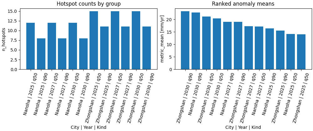
Build one compact visual preview#
This preview is not part of the production builder itself. It is a teaching aid for the gallery page.
- Left:
hotspot counts by city-year-kind.
- Right:
ranked anomaly means.
summary["group"] = (
    summary["city"].astype(str)
    + " | "
    + summary["year"].astype(str)
    + " | "
    + summary["kind"].astype(str)
)

ranked = summary.sort_values(
    ["metric_mean", "n_hotspots"],
    ascending=[False, False],
).reset_index(drop=True)

fig, axes = plt.subplots(
    1,
    2,
    figsize=(10.0, 4.2),
    constrained_layout=True,
)

# Hotspot counts
ax = axes[0]
ax.bar(summary["group"], summary["n_hotspots"])
ax.set_title("Hotspot counts by group")
ax.set_xlabel("City | Year | Kind")
ax.set_ylabel("n_hotspots")
ax.tick_params(axis="x", rotation=75)

# Ranked anomaly means
ax = axes[1]
ax.bar(ranked["group"], ranked["metric_mean"])
ax.set_title("Ranked anomaly means")
ax.set_xlabel("City | Year | Kind")
ax.set_ylabel("metric_mean [mm/yr]")
ax.tick_params(axis="x", rotation=75)
Learn how to read the summary table#
Each row corresponds to one:
city
year
kind
combination.
The core reading order is:
read
n_hotspotsto see how large the hotspot cloud is;read
value_*to understand hotspot subsidence levels;read
metric_*to understand hotspot anomaly intensity;use
baseline_*andthreshold_*when the source CSV provides those optional columns.
In other words:
the point-cloud CSV is the geometric/point-level artifact,
the summary CSV is the compact grouped artifact.
What the key columns mean#
value_*summary of the hotspot subsidence values themselves.
metric_*summary of the anomaly or delta measure used to define or score hotspot points.
baseline_*optional summary of the baseline values attached to the hotspot points.
threshold_*optional summary of the group threshold values.
The threshold is often constant within a group, but the script still keeps both min and max for robustness.
Why this builder is useful in practice#
This builder is a bridge between hotspot maps and later reporting.
A useful workflow is:
generate hotspot points from a spatial forecast workflow,
summarize them by city, year, and kind,
compare counts and anomaly magnitudes across groups,
only then build narrative tables or paper figures.
This keeps:
hotspot extraction,
group-level tabulation,
and final visualization
clearly separated.
Why this page belongs after compute_hotspots.py#
The previous lesson built a compact city-year hotspot table from forecast CSVs directly.
This lesson starts later in the chain:
it assumes hotspot points already exist,
and it compresses those points into grouped summary rows.
So the two scripts are related, but they summarize different intermediate artifacts.
Command-line version#
The same lesson can be reproduced from the CLI.
Legacy dispatcher:
python -m scripts summarize-hotspots \
  --hotspot-csv results/figs/fig6_hotspot_points.csv \
  --out fig6_hotspot_summary.csv
Quiet mode:
python -m scripts summarize-hotspots \
  --hotspot-csv results/figs/fig6_hotspot_points.csv \
  --out fig6_hotspot_summary.csv \
  --quiet true
Modern CLI:
geoprior build hotspots-summary \
  --hotspot-csv results/figs/fig6_hotspot_points.csv \
  --out fig6_hotspot_summary.csv
The gallery page teaches the builder. The command line reproduces it in a workflow.
Total running time of the script: (0 minutes 0.311 seconds)