
Note
Go to the end to download the full example code.
Inspect a Stage-1 manifest before downstream stages#
This lesson teaches how to read a Stage-1 manifest.json
artifact as a workflow handshake.
Why this file matters#
Compared with the Stage-1 audit, the manifest is broader. It answers questions such as:
Which dataset and split settings were actually resolved?
Which columns and feature groups will downstream stages rely on?
Were holdout counts and sequence counts exported?
Which CSV, joblib, and NPZ artifacts were written?
Does the Stage-1 bundle look complete enough for Stage-2?
The goal of this page is not only to produce plots. It is to guide the reader through the file in the order an inspector would normally follow: identity, compact configuration, feature groups, holdout counts, artifact inventory, shape summaries, and final decision checks.
from __future__ import annotations

import json
import tempfile
from pathlib import Path
from pprint import pprint

import matplotlib.pyplot as plt
import pandas as pd

from geoprior.utils.inspect import (
    generate_manifest,
    inspect_manifest,
    load_manifest,
    manifest_artifacts_frame,
    manifest_config_frame,
    manifest_feature_groups_frame,
    manifest_holdout_frame,
    manifest_identity_frame,
    manifest_paths_frame,
    manifest_shapes_frame,
    manifest_versions_frame,
    plot_manifest_artifact_inventory,
    plot_manifest_boolean_summary,
    plot_manifest_coord_ranges,
    plot_manifest_feature_group_sizes,
    plot_manifest_holdout_counts,
    summarize_manifest,
)

pd.set_option("display.max_columns", 24)
pd.set_option("display.width", 110)


MANIFEST_PALETTE = {
    "inventory": "#4C6EF5",
    "features": "#0F766E",
    "holdout": "#C2410C",
    "coords": "#7C3AED",
    "pass": "#15803D",
    "fail": "#B91C1C",
    "edge": "#243B53",
    "panel": "#FBFCFE",
}


def _style_bar_panel(
    ax: plt.Axes,
    *,
    color: str,
    edge: str = MANIFEST_PALETTE["edge"],
) -> None:
    """Polish a bar-based gallery panel."""
    for patch in ax.patches:
        patch.set_facecolor(color)
        patch.set_edgecolor(edge)
        patch.set_linewidth(1.25)
        patch.set_alpha(0.94)
    ax.set_facecolor(MANIFEST_PALETTE["panel"])
    ax.tick_params(labelsize=9)
    ax.title.set_fontweight("bold")
    for side in ("top", "right"):
        ax.spines[side].set_visible(False)
    for side in ("left", "bottom"):
        ax.spines[side].set_color("#CBD5E1")


def _style_boolean_panel(ax: plt.Axes) -> None:
    """Apply a distinct pass/fail palette to boolean panels."""
    for patch in ax.patches:
        width = patch.get_width()
        height = patch.get_height()
        score = width if width != 0 else height
        color = (
            MANIFEST_PALETTE["pass"]
            if score >= 0.5
            else MANIFEST_PALETTE["fail"]
        )
        patch.set_facecolor(color)
        patch.set_edgecolor(MANIFEST_PALETTE["edge"])
        patch.set_linewidth(1.15)
        patch.set_alpha(0.94)
    ax.set_facecolor("#FCFCFD")
    ax.tick_params(labelsize=9)
    ax.title.set_fontweight("bold")
    for side in ("top", "right"):
        ax.spines[side].set_visible(False)
    for side in ("left", "bottom"):
        ax.spines[side].set_color("#CBD5E1")
What this lesson will teach#
We will inspect the manifest in a deliberate workflow order:
confirm what artifact we are opening,
read the compact summary,
inspect the run identity and compact config,
inspect feature groups and holdout counts,
inspect artifact paths and runtime versions,
inspect the saved tensor-shape summary,
use the boolean checks as a final decision panel.
This order matters because the manifest is a workflow contract. Before caring about fine details, we want to know whether the file is structurally complete enough to support downstream steps.
Create a realistic demo manifest#
For a gallery lesson, a stable synthetic-but-realistic manifest is usually better than re-running the whole preprocessing pipeline. The helper below creates such a file while preserving the broad structure of a real Stage-1 manifest.
In real work, you would simply point these inspection helpers to the
manifest written under your own results/... directory.
out_dir = Path(tempfile.mkdtemp(prefix="gp_manifest_"))
manifest_path = out_dir / "manifest.json"

generate_manifest(
    manifest_path,
    overrides={
        "city": "nansha",
        "model": "GeoPriorSubsNet",
        "timestamp": "2026-03-28 13:41:18",
        "config": {
            "TIME_STEPS": 5,
            "FORECAST_HORIZON_YEARS": 3,
            "MODE": "tft_like",
            "TRAIN_END_YEAR": 2022,
            "FORECAST_START_YEAR": 2023,
        },
    },
)

print("Written manifest file")
print(f" - {manifest_path}")
Written manifest file
 - /tmp/gp_manifest_au38nzac/manifest.json
Load the manifest with the real reader#
The inspection path should look as close as possible to real usage,
so we load the file through load_manifest(...) rather than
treating it as a plain JSON blob.
manifest_record = load_manifest(manifest_path)

print("\nArtifact header")
pprint(
    {
        "kind": manifest_record.kind,
        "stage": manifest_record.stage,
        "city": manifest_record.city,
        "model": manifest_record.model,
        "path": str(manifest_record.path),
    }
)
Artifact header
{'city': 'nansha',
 'kind': 'manifest',
 'model': 'GeoPriorSubsNet',
 'path': '/tmp/gp_manifest_au38nzac/manifest.json',
 'stage': 'stage1'}
Start with the compact summary#
The summary is the best first stop because it compresses the broad manifest into a quick decision-oriented overview.
It answers questions such as:
how many feature groups were recorded,
whether scaling kwargs and holdout metadata exist,
how many artifact paths and top-level paths were saved,
and whether core sections such as
configandversionsare present.
summary = summarize_manifest(manifest_record)

print("\nCompact summary")
print(json.dumps(summary, indent=2))
Compact summary
{
  "schema_version": "3.2",
  "timestamp": "2026-03-28 13:41:18",
  "stage": "stage1",
  "city": "nansha",
  "model": "GeoPriorSubsNet",
  "time_steps": 5,
  "forecast_horizon_years": 3,
  "mode": "tft_like",
  "train_end_year": 2022,
  "forecast_start_year": 2023,
  "static_feature_count": 12,
  "dynamic_feature_count": 5,
  "future_feature_count": 1,
  "group_id_cols_count": 2,
  "coord_ranges": {
    "t": 7.0,
    "x": 44447.0,
    "y": 39275.0
  },
  "artifact_path_count": 14,
  "path_count": 2,
  "version_count": 5,
  "train_groups": 136351,
  "val_groups": 38958,
  "test_groups": 19479,
  "train_rows": 1090808,
  "val_rows": 311664,
  "test_rows": 155832,
  "train_seq": 136351,
  "val_seq": 38958,
  "test_seq": 19479,
  "has_config": true,
  "has_artifacts": true,
  "has_paths": true,
  "has_versions": true,
  "has_holdout": true,
  "has_scaling_kwargs": true
}
Interpret the summary before digging deeper#
A lesson should not stop at printing the summary. We also want to interpret it.
In a real workflow, this is the stage where a user asks whether the manifest seems complete enough to deserve deeper reading.
print("\nInterpretation of the summary")
print(
    "- Feature-group sizes:",
    {
        "static": summary.get("static_feature_count"),
        "dynamic": summary.get("dynamic_feature_count"),
        "future": summary.get("future_feature_count"),
        "group_id_cols": summary.get("group_id_cols_count"),
    },
)
print(
    "- Inventory counts:",
    {
        "artifact_paths": summary.get("artifact_path_count"),
        "paths": summary.get("path_count"),
        "versions": summary.get("version_count"),
    },
)
print(
    "- Split counts:",
    {
        "train_groups": summary.get("train_groups"),
        "val_groups": summary.get("val_groups"),
        "test_groups": summary.get("test_groups"),
        "train_seq": summary.get("train_seq"),
        "val_seq": summary.get("val_seq"),
        "test_seq": summary.get("test_seq"),
    },
)
Interpretation of the summary
- Feature-group sizes: {'static': 12, 'dynamic': 5, 'future': 1, 'group_id_cols': 2}
- Inventory counts: {'artifact_paths': 14, 'paths': 2, 'versions': 5}
- Split counts: {'train_groups': 136351, 'val_groups': 38958, 'test_groups': 19479, 'train_seq': 136351, 'val_seq': 38958, 'test_seq': 19479}
Inspect the identity and compact config#
The identity frame is the first place to check whether we are looking at the file we think we are looking at.
The compact config frame then answers a different question: what high-level settings actually governed Stage-1?
identity = manifest_identity_frame(manifest_record)
config_frame = manifest_config_frame(manifest_record)

print("\nIdentity view")
print(identity)

print("\nCompact config view")
print(config_frame)
Identity view
    section             key                value
0  identity  schema_version                  3.2
1  identity       timestamp  2026-03-28 13:41:18
2  identity           stage               stage1
3  identity            city               nansha
4  identity           model      GeoPriorSubsNet

Compact config view
        section                     key                                   value
0        config              TIME_STEPS                                       5
1        config  FORECAST_HORIZON_YEARS                                       3
2        config                    MODE                                tft_like
3        config          TRAIN_END_YEAR                                    2022
4        config     FORECAST_START_YEAR                                    2023
5   conventions                gwl_kind                               depth_bgs
6   conventions                gwl_sign                           down_positive
7   conventions          use_head_proxy                                   False
8   conventions              time_units                                    year
9   conventions         gwl_driver_kind                                   depth
10  conventions         gwl_target_kind                                    head
11       config            coord_ranges  {'t': 7.0, 'x': 44447.0, 'y': 39275.0}
Why the compact config matters#
These few values often explain later workflow behavior. For example:
TIME_STEPSandFORECAST_HORIZON_YEARSshape the sequence layout,MODEhelps explain how downstream tensors are organized,TRAIN_END_YEARandFORECAST_START_YEARprovide temporal context for the split.
A mismatch here can explain many later surprises.
Inspect feature groups and holdout counts#
After identity and config, the next practical question is whether the data organization looks plausible.
The feature-group frame tells us what kinds of information were exported. The holdout frame tells us whether the split sizes look coherent enough for later stages.
feature_groups = manifest_feature_groups_frame(manifest_record)
holdout = manifest_holdout_frame(manifest_record)

print("\nFeature groups")
print(feature_groups.loc[:, ["group", "count", "values"]])

print("\nHoldout and split counts")
print(holdout)
Feature groups
           group  count                                             values
0         static     12  [lithology_Conglomerate–Sandstone, lithology_L...
1        dynamic      5  [GWL_depth_bgs_m__si, subsidence_cum__si, rain...
2         future      1                                      [rainfall_mm]
3  group_id_cols      2                              [longitude, latitude]

Holdout and split counts
            section                  key    value
0      group_counts      valid_for_train   194788
1      group_counts   valid_for_forecast   194788
2      group_counts  kept_for_processing   194788
3      group_counts         train_groups   136351
4      group_counts           val_groups    38958
5      group_counts          test_groups    19479
6   row_counts_hist           train_rows  1090808
7   row_counts_hist             val_rows   311664
8   row_counts_hist            test_rows   155832
9   sequence_counts            train_seq   136351
10  sequence_counts              val_seq    38958
11  sequence_counts             test_seq    19479
12     holdout_meta             strategy   random
13     holdout_meta                 seed       42
14     holdout_meta             val_frac 0.200000
15     holdout_meta            test_frac 0.100000
Interpret the feature groups and holdout counts#
A strong inspection habit is to convert these tables into a short narrative rather than treating them as passive output.
print("\nInterpretation of feature groups")
for _, row in feature_groups.iterrows():
    print(f"- {row['group']}: {row['count']} entries")

holdout_map = dict(zip(holdout["key"], holdout["value"], strict=False))
print("\nInterpretation of holdout structure")
print(
    "- Group counts suggest how many spatial / logical groups are "
    "present in each split."
)
print(
    "- Sequence counts indicate how many sequence samples were "
    "actually exported for training and validation."
)
print(
    "- A very small validation or test split would deserve a closer "
    "look before trusting later metrics."
)
print(
    "- Current values:",
    {
        key: holdout_map.get(key)
        for key in [
            "train_groups",
            "val_groups",
            "test_groups",
            "train_seq",
            "val_seq",
            "test_seq",
        ]
    },
)
Interpretation of feature groups
- static: 12 entries
- dynamic: 5 entries
- future: 1 entries
- group_id_cols: 2 entries

Interpretation of holdout structure
- Group counts suggest how many spatial / logical groups are present in each split.
- Sequence counts indicate how many sequence samples were actually exported for training and validation.
- A very small validation or test split would deserve a closer look before trusting later metrics.
- Current values: {'train_groups': 136351, 'val_groups': 38958, 'test_groups': 19479, 'train_seq': 136351, 'val_seq': 38958, 'test_seq': 19479}
Inspect artifact, path, version, and shape inventories#
This is the part that makes the manifest especially valuable as a downstream handshake.
It tells us:
what Stage-1 actually wrote,
where those outputs live,
what runtime versions were recorded,
and what the exported tensors look like structurally.
artifacts = manifest_artifacts_frame(manifest_record)
paths = manifest_paths_frame(manifest_record)
versions = manifest_versions_frame(manifest_record)
shapes = manifest_shapes_frame(manifest_record)

print("\nArtifact inventory (first rows)")
print(artifacts.head(18))

print("\nTop-level paths")
print(paths)

print("\nRuntime versions")
print(versions)

print("\nTensor shape summary")
print(shapes.head(12))
Artifact inventory (first rows)
      section                                   key                                              value  \
0   artifacts                               csv.raw  results/nansha_GeoPriorSubsNet_stage1/nansha_0...
1   artifacts                             csv.clean  results/nansha_GeoPriorSubsNet_stage1/nansha_0...
2   artifacts                            csv.scaled  results/nansha_GeoPriorSubsNet_stage1/nansha_0...
3   artifacts                encoders.ohe.lithology  results/nansha_GeoPriorSubsNet_stage1/artifact...
4   artifacts          encoders.ohe.lithology_class  results/nansha_GeoPriorSubsNet_stage1/artifact...
5   artifacts                 encoders.coord_scaler  results/nansha_GeoPriorSubsNet_stage1/artifact...
6   artifacts                  encoders.main_scaler  results/nansha_GeoPriorSubsNet_stage1/artifact...
7   artifacts       encoders.scaled_ml_numeric_cols             [rainfall_mm, soil_thickness_censored]
8   artifacts      sequences.joblib_train_sequences  results/nansha_GeoPriorSubsNet_stage1/artifact...
9   artifacts  sequences.dims.output_subsidence_dim                                                  1
10  artifacts         sequences.dims.output_gwl_dim                                                  1
11  artifacts                numpy.train_inputs_npz  results/nansha_GeoPriorSubsNet_stage1/artifact...
12  artifacts               numpy.train_targets_npz  results/nansha_GeoPriorSubsNet_stage1/artifact...
13  artifacts                  numpy.val_inputs_npz  results/nansha_GeoPriorSubsNet_stage1/artifact...
14  artifacts                 numpy.val_targets_npz  results/nansha_GeoPriorSubsNet_stage1/artifact...
15  artifacts                 numpy.test_inputs_npz  results/nansha_GeoPriorSubsNet_stage1/artifact...
16  artifacts                numpy.test_targets_npz  results/nansha_GeoPriorSubsNet_stage1/artifact...
17  artifacts           shapes.train_inputs.H_field                                     [136351, 3, 1]

                               basename  is_path
0                     nansha_01_raw.csv     True
1                   nansha_02_clean.csv     True
2                  nansha_03_scaled.csv     True
3           nansha_ohe_lithology.joblib     True
4     nansha_ohe_lithology_class.joblib     True
5            nansha_coord_scaler.joblib     True
6             nansha_main_scaler.joblib     True
7                                   NaN    False
8   nansha_train_sequences_T5_H3.joblib     True
9                                   NaN    False
10                                  NaN    False
11                     train_inputs.npz     True
12                    train_targets.npz     True
13                       val_inputs.npz     True
14                      val_targets.npz     True
15                      test_inputs.npz     True
16                     test_targets.npz     True
17                                  NaN    False

Top-level paths
  section            key                                            value                       basename
0   paths        run_dir            results/nansha_GeoPriorSubsNet_stage1  nansha_GeoPriorSubsNet_stage1
1   paths  artifacts_dir  results/nansha_GeoPriorSubsNet_stage1/artifacts                      artifacts

Runtime versions
    section         key    value
0  versions      python  3.10.19
1  versions  tensorflow   2.20.0
2  versions       numpy    2.0.2
3  versions      pandas    2.3.3
4  versions     sklearn    1.7.2

Tensor shape summary
            split            tensor           shape  rank  samples  time_dim  feature_dim
0    train_inputs           H_field  [136351, 3, 1]     3   136351         3     1.000000
1    train_inputs            coords  [136351, 3, 3]     3   136351         3     3.000000
2    train_inputs  dynamic_features  [136351, 5, 5]     3   136351         5     5.000000
3    train_inputs   future_features  [136351, 8, 1]     3   136351         8     1.000000
4    train_inputs   static_features    [136351, 12]     2   136351        12          NaN
5   train_targets          gwl_pred  [136351, 3, 1]     3   136351         3     1.000000
6   train_targets         subs_pred  [136351, 3, 1]     3   136351         3     1.000000
7      val_inputs           H_field   [38958, 3, 1]     3    38958         3     1.000000
8      val_inputs            coords   [38958, 3, 3]     3    38958         3     3.000000
9      val_inputs  dynamic_features   [38958, 5, 5]     3    38958         5     5.000000
10     val_inputs   future_features   [38958, 8, 1]     3    38958         8     1.000000
11     val_inputs   static_features     [38958, 12]     2    38958        12          NaN
How to read the inventory sections#
These sections answer slightly different questions:
the artifact inventory says what was exported,
the path table says where it was exported,
the version table says with which software context,
the shape table says what tensor layouts downstream code should expect.
When something later fails in Stage-2, the shape table is often one of the most useful places to revisit.
Use the all-in-one inspector#
inspect_manifest(...) is convenient when a workflow or CLI
helper wants the normalized payload, summary, and main tidy frames
in one call.
Inspector bundle keys
['artifacts', 'config', 'feature_groups', 'holdout', 'identity', 'paths', 'payload', 'shapes', 'summary', 'versions']
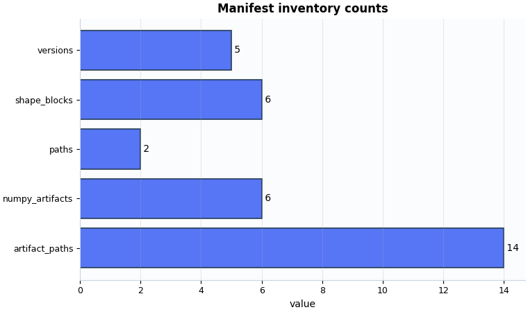
Plot 1: artifact inventory#
This plot is a compact answer to the question:
Did Stage-1 actually export the bundle we expect?
What to look for:
at least some artifact paths should exist,
the path and version counts should not be empty,
numpy / shape blocks should exist when later stages depend on them.
fig, ax = plt.subplots(
    figsize=(7.6, 4.5),
    constrained_layout=True,
)
plot_manifest_artifact_inventory(
    ax,
    manifest_record,
    title="Manifest inventory counts",
)
_style_bar_panel(ax, color=MANIFEST_PALETTE["inventory"])
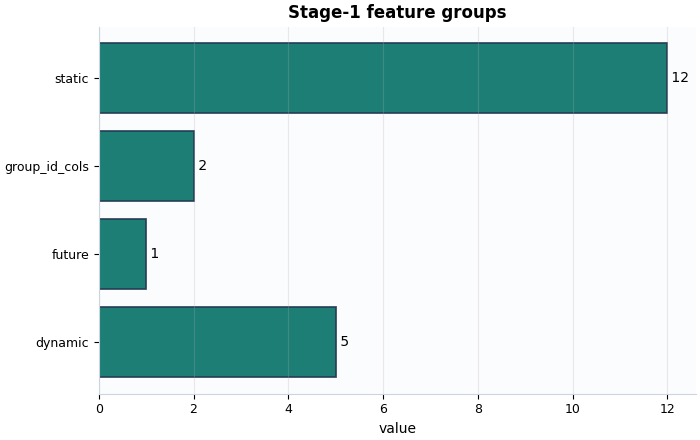
Plot 2: feature-group sizes#
This plot makes the feature composition readable at a glance.
What to look for:
static, dynamic, and future groups should all be present when your workflow expects them,
group-id columns should not silently disappear,
a missing future group may explain later forecasting issues.
fig, ax = plt.subplots(
    figsize=(7.0, 4.4),
    constrained_layout=True,
)
plot_manifest_feature_group_sizes(
    ax,
    manifest_record,
    title="Stage-1 feature groups",
)
_style_bar_panel(ax, color=MANIFEST_PALETTE["features"])
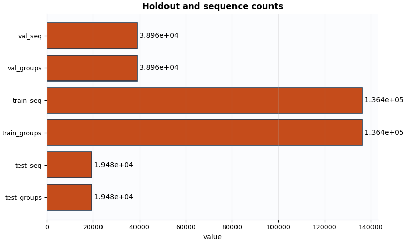
Plot 3: holdout and sequence counts#
This plot helps answer whether the split sizes look balanced enough for the next workflow step.
What to look for:
train counts should usually dominate,
validation and test counts should not be accidentally tiny,
sequence counts should not collapse to zero.
fig, ax = plt.subplots(
    figsize=(8.0, 4.8),
    constrained_layout=True,
)
plot_manifest_holdout_counts(
    ax,
    manifest_record,
    title="Holdout and sequence counts",
)
_style_bar_panel(ax, color=MANIFEST_PALETTE["holdout"])
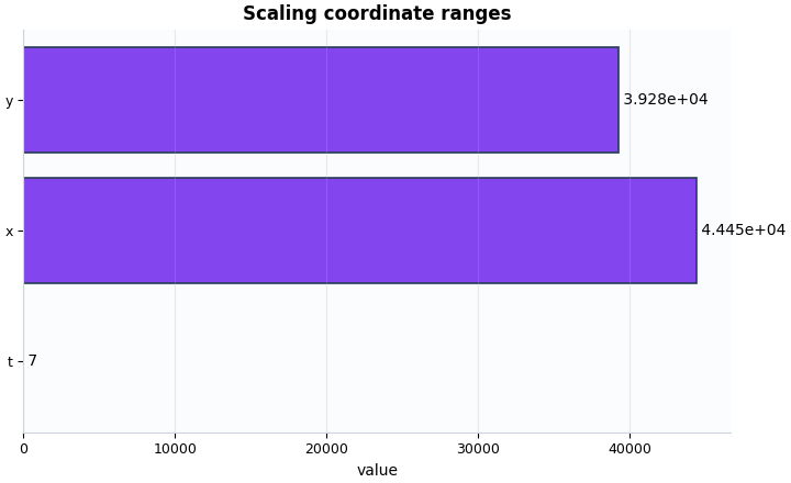
Plot 4: coordinate ranges from scaling kwargs#
Even though the manifest is broader than the Stage-1 audit, it still carries important scaling context. These ranges remind the user that the manifest also preserves downstream conventions, not only file paths.
What to look for:
ranges should be positive,
values should be plausible for the dataset extent,
the presence of this block confirms that scaling metadata was exported into the Stage-1 handshake.
fig, ax = plt.subplots(
    figsize=(7.2, 4.4),
    constrained_layout=True,
)
plot_manifest_coord_ranges(
    ax,
    manifest_record,
    title="Scaling coordinate ranges",
)
_style_bar_panel(ax, color=MANIFEST_PALETTE["coords"])
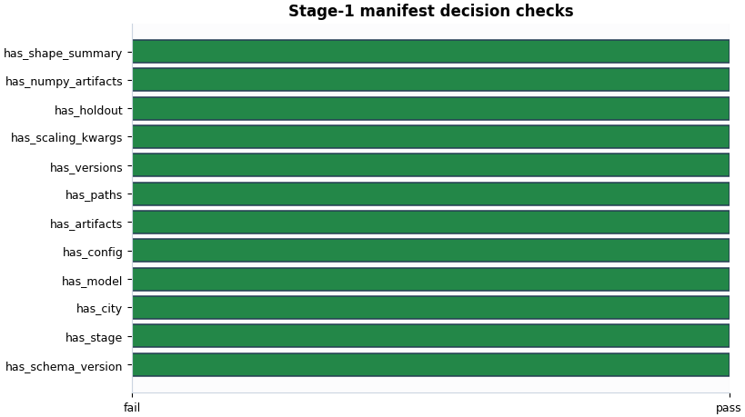
Plot 5: structural decision checks#
This boolean summary works like a final gate.
It does not replace the detailed reading above, but it provides a fast answer to the question:
Does this manifest contain the core sections a downstream stage would expect?
fig, ax = plt.subplots(
    figsize=(8.2, 4.6),
    constrained_layout=True,
)
plot_manifest_boolean_summary(
    ax,
    manifest_record,
    title="Stage-1 manifest decision checks",
)
_style_boolean_panel(ax)
Final reading rule#
A simple lesson-level decision rule for a Stage-1 manifest is:
schema and stage are present,
config / artifacts / paths / versions are present,
holdout and scaling kwargs exist,
at least one real artifact path was recorded.
When these checks pass, the manifest usually looks healthy enough to trust as a Stage-1 handshake for later steps.
must_pass = [
    "has_config",
    "has_artifacts",
    "has_paths",
    "has_versions",
    "has_holdout",
    "has_scaling_kwargs",
]
ready = all(bool(summary.get(name, False)) for name in must_pass)
ready = ready and int(summary.get("artifact_path_count", 0) or 0) > 0

print("\nDecision note")
if ready:
    print(
        "This manifest looks structurally complete enough to support "
        "downstream workflow stages."
    )
else:
    print(
        "This manifest deserves more attention before you rely on it "
        "downstream."
    )
Decision note
This manifest looks structurally complete enough to support downstream workflow stages.
Total running time of the script: (0 minutes 0.529 seconds)