Plot epsilon diagnostics from a GeoPrior training history

This example teaches you how to use GeoPrior’s plot_epsilons_in helper.

Unlike the paper-oriented scripts in figure_generation/, this function is a compact model-inspection utility. It focuses only on the epsilon-style physics diagnostics stored in a training history.

Why this matters

GeoPrior histories can contain many keys, but the epsilon terms are often the quickest way to inspect whether physics residual diagnostics are shrinking, stabilizing, or oscillating during training.

This helper makes that easy because it:

• selects only epsilon_* keys,

• ignores unrelated history terms,

• plots them in one compact panel,

• and uses safe log-like scaling.

Imports

We call the real plotting helper from the package and feed it a compact synthetic history dictionary.

from __future__ import annotations

import tempfile
from pathlib import Path

import numpy as np

from geoprior.models import plot_epsilons_in

Build a compact synthetic history

The real helper accepts a Keras History or a plain dict. For the lesson page, a plain dict is enough.

We include:

• epsilon diagnostics that should be plotted,

• other loss keys that should be ignored by this helper,

• one epsilon series that crosses zero so the requested log scale will safely fall back to symlog.

epochs = np.arange(1, 13, dtype=int)

history = {
    "loss": (
        np.array(
            [2.2, 1.8, 1.45, 1.18, 0.98, 0.84, 0.75, 0.69,
             0.64, 0.60, 0.57, 0.55]
        )
    ).tolist(),
    "physics_loss": (
        np.array(
            [0.80, 0.63, 0.49, 0.37, 0.29, 0.23, 0.19, 0.16,
             0.14, 0.13, 0.12, 0.11]
        )
    ).tolist(),
    "epsilon_prior": (
        np.array(
            [0.24, 0.18, 0.13, 0.095, 0.070, 0.050,
             0.034, 0.020, 0.011, 0.006, 0.003, 0.0015]
        )
    ).tolist(),
    "epsilon_cons": (
        np.array(
            [0.18, 0.145, 0.11, 0.085, 0.062, 0.044,
             0.028, 0.016, 0.009, 0.005, 0.002, 0.001]
        )
    ).tolist(),
    "epsilon_gw": (
        np.array(
            [0.12, 0.10, 0.08, 0.060, 0.045, 0.031,
             0.020, 0.010, 0.004, 0.000, -0.002, 0.001]
        )
    ).tolist(),
    "epsilon_cons_raw": (
        np.array(
            [0.30, 0.24, 0.19, 0.15, 0.11, 0.085,
             0.060, 0.040, 0.023, 0.012, 0.007, 0.004]
        )
    ).tolist(),
    "epsilon_gw_raw": (
        np.array(
            [0.22, 0.18, 0.14, 0.11, 0.085, 0.063,
             0.042, 0.022, 0.010, 0.004, 0.001, 0.0005]
        )
    ).tolist(),
}

print("History keys")
for k in history:
    print(" -", k)

History keys
 - loss
 - physics_loss
 - epsilon_prior
 - epsilon_cons
 - epsilon_gw
 - epsilon_cons_raw
 - epsilon_gw_raw

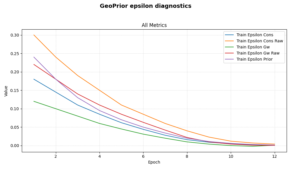
Plot the epsilon dashboard directly

The helper automatically:

• extracts non-validation epsilon_* keys,

• groups them into one panel called Epsilons,

• requests log-like scaling.

Because epsilon_gw touches zero and becomes slightly negative, the underlying history plotter will safely use symlog instead of a strict log scale.

plot_epsilons_in(
    history,
    title="GeoPrior epsilon diagnostics",
    style="default",
)

Save the epsilon figure

When savefig has no extension, the underlying plot helper adds .png automatically.

tmp_dir = Path(
    tempfile.mkdtemp(prefix="gp_sg_plot_epsilons_")
)
save_stem = tmp_dir / "epsilon_dashboard"

plot_epsilons_in(
    history,
    title="Saved epsilon diagnostics",
    savefig=str(save_stem),
)

saved_png = tmp_dir / "epsilon_dashboard.png"

print("")
print("Saved file")
print(" -", saved_png)

[OK] Saved figure -> /tmp/gp_sg_plot_epsilons_6phk19qe/epsilon_dashboard.png

Saved file
 - /tmp/gp_sg_plot_epsilons_6phk19qe/epsilon_dashboard.png

Show what the helper is selecting

This helper is intentionally narrow: it ignores losses and only cares about keys beginning with epsilon_.

selected = sorted(
    [k for k in history if k.startswith("epsilon_")]
)

print("")
print("Selected epsilon keys")
for k in selected:
    print(" -", k)

Selected epsilon keys
 - epsilon_cons
 - epsilon_cons_raw
 - epsilon_gw
 - epsilon_gw_raw
 - epsilon_prior

Learn how to read the epsilon panel

A useful reading order is:

1. compare epsilon_prior against the PDE-style epsilons;

2. inspect whether all epsilon terms shrink together or whether one residual family plateaus;

3. inspect *_raw terms separately when you want to compare the scaled and unscaled versions of a residual family.

This is why a dedicated epsilon plot is often clearer than a full all-metrics dashboard.

Why safe symlog matters here

Epsilon diagnostics can get very small, touch zero, or even cross zero depending on how they are logged.

A strict log axis would be brittle in that case. This helper instead requests log scaling and lets the base history plotter fall back to symlog when needed.

That keeps the panel readable even near zero.

Why this page belongs in model_inspection

This helper is not building a publication figure and it is not exporting a reusable artifact.

Its job is to inspect the training dynamics of the physics diagnostics themselves.

So it belongs naturally with the other model-inspection helpers.

A natural next lesson

The clean next page after this is plot_physics_losses_in.py, because it is the sister helper that focuses on physics loss terms instead of epsilon diagnostics.