
Note
Go to the end to download the full example code.
External validation of inferred effective fields#
This application turns the Zhongshan point-support validation into a practical reading page.
The scientific question is straightforward:
Do the learned effective fields remain anchored to independent site evidence, or are they only internally self-consistent?
The page focuses on the five Zhongshan borehole and pumping-test sites used for independent checking of the thickness and conductivity pathways.
What this application shows#
The thickness pathway receives independent support through a positive rank association between borehole-derived thickness and collocated model \(H_{\mathrm{eff}}\).
The same comparison also shows why \(H_{\mathrm{eff}}\) should be read as a capped effective thickness field rather than as an uncensored borehole-thickness estimator.
Pumping-test productivity provides only weak direct support for cell-scale \(K\), so conductivity maps should be read more cautiously than the thickness pathway.
Why this matters#
A physics-guided model becomes much more credible when at least part of its internal structure aligns with field information that was not used as a direct training target. This page therefore complements the forecasting, identifiability, hotspot, and transfer applications by showing where external anchoring is strong and where it remains limited.
from __future__ import annotations

import numpy as np
import pandas as pd
import matplotlib.pyplot as plt


CITY_COLOR = "#d7301f"
THICKNESS_COLOR = "#3182bd"
K_COLOR = "#756bb1"
CAP_THICKNESS_M = 30.0


def build_site_table() -> pd.DataFrame:
    """Return the compact Zhongshan validation table.

    The values are the application-ready site summaries reported for
    the five external-validation locations used in the Zhongshan case
    study.
    """
    rows = [
        {
            "site": "SW1",
            "x": 738471.86,
            "y": 2503364.59,
            "borehole_thickness_m": 50.4,
            "model_heff_m": 30.0,
            "model_hd_m": 18.0,
            "model_k_mps": 3.24e-12,
            "specific_capacity_ls_per_m": 0.105,
            "match_distance_m": 14.3,
        },
        {
            "site": "SW2",
            "x": 740742.92,
            "y": 2500323.08,
            "borehole_thickness_m": 27.7,
            "model_heff_m": 30.0,
            "model_hd_m": 18.0,
            "model_k_mps": 3.20e-12,
            "specific_capacity_ls_per_m": 0.306,
            "match_distance_m": 163.0,
        },
        {
            "site": "SW3",
            "x": 745780.54,
            "y": 2499975.34,
            "borehole_thickness_m": 43.0,
            "model_heff_m": 30.0,
            "model_hd_m": 18.0,
            "model_k_mps": 3.41e-12,
            "specific_capacity_ls_per_m": 0.785,
            "match_distance_m": 15.4,
        },
        {
            "site": "SW4",
            "x": 749332.53,
            "y": 2503557.96,
            "borehole_thickness_m": 22.5,
            "model_heff_m": 3.0,
            "model_hd_m": 1.8,
            "model_k_mps": 3.87e-12,
            "specific_capacity_ls_per_m": 0.199,
            "match_distance_m": 86.1,
        },
        {
            "site": "SW5",
            "x": 754049.13,
            "y": 2500176.54,
            "borehole_thickness_m": 35.1,
            "model_heff_m": 30.0,
            "model_hd_m": 18.0,
            "model_k_mps": 3.94e-12,
            "specific_capacity_ls_per_m": 0.186,
            "match_distance_m": 41.1,
        },
    ]
    df = pd.DataFrame(rows)
    df["thickness_residual_m"] = (
        df["model_heff_m"] - df["borehole_thickness_m"]
    )
    return df


def build_summary(df: pd.DataFrame) -> pd.Series:
    """Summarize the external-validation message.

    Positive rank support for the thickness pathway is quantified by
    the Spearman association between borehole thickness and model
    ``Heff``. Conductivity support is represented by the association
    between late-step specific capacity and model ``K``.
    """
    rho_heff = df[
        ["borehole_thickness_m", "model_heff_m"]
    ].corr(method="spearman").iloc[0, 1]

    rho_k = df[
        ["specific_capacity_ls_per_m", "model_k_mps"]
    ].corr(method="spearman").iloc[0, 1]

    return pd.Series(
        {
            "n_sites": int(len(df)),
            "rho_heff": float(rho_heff),
            "mae_heff_m": float(
                (df["thickness_residual_m"]).abs().mean()
            ),
            "median_bias_heff_m": float(
                df["thickness_residual_m"].median()
            ),
            "rho_k": float(rho_k),
            "median_match_distance_m": float(
                df["match_distance_m"].median()
            ),
            "min_match_distance_m": float(
                df["match_distance_m"].min()
            ),
            "max_match_distance_m": float(
                df["match_distance_m"].max()
            ),
        }
    )


sites = build_site_table()
summary = build_summary(sites)
Problem framing#
The forecasting story is stronger when internal physics fields are checked against independent site information. In this study, that anchor is available only in Zhongshan, where five borehole logs are co-located with step-drawdown pumping tests.
This application is intentionally narrow. It does not try to turn sparse site evidence into a universal truth test. Instead, it asks a more precise question:
does the thickness pathway track independent field ordering,
where does the capped representation bias absolute thickness,
and how much direct support do the sparse pumping tests provide for cell-scale conductivity?
That is the right level of ambition for a reduced-physics external validation.
print("Zhongshan validation sites:\n")
print(
    sites[
        [
            "site",
            "borehole_thickness_m",
            "model_heff_m",
            "model_hd_m",
            "model_k_mps",
            "specific_capacity_ls_per_m",
            "match_distance_m",
        ]
    ]
    .round(
        {
            "borehole_thickness_m": 1,
            "model_heff_m": 1,
            "model_hd_m": 1,
            "model_k_mps": 14,
            "specific_capacity_ls_per_m": 3,
            "match_distance_m": 1,
        }
    )
    .to_string(index=False)
)

print("\nApplication summary:\n")
print(summary.round(3).to_string())
Zhongshan validation sites:

site  borehole_thickness_m  model_heff_m  model_hd_m  model_k_mps  specific_capacity_ls_per_m  match_distance_m
 SW1                  50.4          30.0        18.0 3.240000e-12                       0.105              14.3
 SW2                  27.7          30.0        18.0 3.200000e-12                       0.306             163.0
 SW3                  43.0          30.0        18.0 3.410000e-12                       0.785              15.4
 SW4                  22.5           3.0         1.8 3.870000e-12                       0.199              86.1
 SW5                  35.1          30.0        18.0 3.940000e-12                       0.186              41.1

Application summary:

n_sites                      5.000
rho_heff                     0.707
mae_heff_m                  12.060
median_bias_heff_m         -13.000
rho_k                       -0.200
median_match_distance_m     41.100
min_match_distance_m        14.300
max_match_distance_m       163.000
Rebuild the external-validation application view#
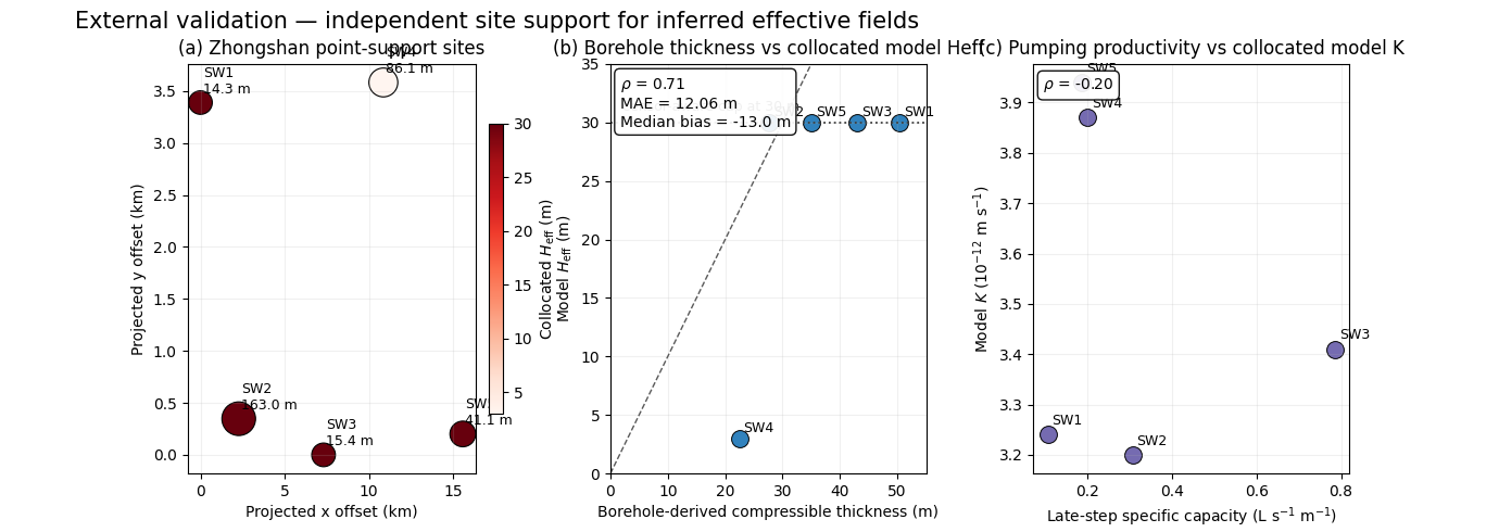
The first panel shows where the five validation sites sit inside the Zhongshan domain. The second tests the thickness pathway directly. The third asks whether pumping productivity aligns with model K. The last panel explains how to read the result safely.
fig = plt.figure(figsize=(13.8, 4.9))
grid = fig.add_gridspec(1, 3, wspace=0.34)

ax_a = fig.add_subplot(grid[0, 0])
ax_b = fig.add_subplot(grid[0, 1])
ax_c = fig.add_subplot(grid[0, 2])


# Panel (a): site-support map
x_km = (sites["x"] - sites["x"].min()) / 1000.0
y_km = (sites["y"] - sites["y"].min()) / 1000.0
size = 220 + 1.7 * sites["match_distance_m"]

sc = ax_a.scatter(
    x_km,
    y_km,
    c=sites["model_heff_m"],
    s=size,
    cmap="Reds",
    edgecolor="black",
    linewidth=0.8,
)

for _, row in sites.iterrows():
    ax_a.text(
        (row["x"] - sites["x"].min()) / 1000.0 + 0.15,
        (row["y"] - sites["y"].min()) / 1000.0 + 0.06,
        f"{row['site']}\n{row['match_distance_m']:.1f} m",
        fontsize=9,
        ha="left",
        va="bottom",
    )

cb = plt.colorbar(sc, ax=ax_a, fraction=0.046, pad=0.04)
cb.set_label(r"Collocated $H_{\mathrm{eff}}$ (m)")
ax_a.set_title("(a) Zhongshan point-support sites")
ax_a.set_xlabel("Projected x offset (km)")
ax_a.set_ylabel("Projected y offset (km)")
ax_a.grid(alpha=0.18)


# Panel (b): thickness pathway
ax_b.scatter(
    sites["borehole_thickness_m"],
    sites["model_heff_m"],
    s=130,
    color=THICKNESS_COLOR,
    edgecolor="black",
    linewidth=0.7,
)

for _, row in sites.iterrows():
    ax_b.text(
        row["borehole_thickness_m"] + 0.7,
        row["model_heff_m"] + 0.5,
        row["site"],
        fontsize=9,
    )

line = np.linspace(0.0, 55.0, 200)
ax_b.plot(line, line, linestyle="--", linewidth=1.0, color="0.35")
ax_b.axhline(
    CAP_THICKNESS_M,
    linestyle=":",
    linewidth=1.3,
    color="0.25",
)
ax_b.text(
    2.0,
    CAP_THICKNESS_M + 1.0,
    "censor-aware cap at 30 m",
    fontsize=9,
    color="0.25",
)
ax_b.set_title("(b) Borehole thickness vs collocated model Heff")
ax_b.set_xlabel("Borehole-derived compressible thickness (m)")
ax_b.set_ylabel(r"Model $H_{\mathrm{eff}}$ (m)")
ax_b.set_xlim(0.0, 55.0)
ax_b.set_ylim(0.0, 35.0)
ax_b.grid(alpha=0.18)

ax_b.text(
    0.03,
    0.97,
    (
        fr"$\rho$ = {summary['rho_heff']:.2f}" "\n"
        fr"MAE = {summary['mae_heff_m']:.2f} m" "\n"
        fr"Median bias = {summary['median_bias_heff_m']:.1f} m"
    ),
    transform=ax_b.transAxes,
    ha="left",
    va="top",
    bbox=dict(boxstyle="round,pad=0.35", facecolor="white", alpha=0.92),
)


# Panel (c): conductivity proxy support
ax_c.scatter(
    sites["specific_capacity_ls_per_m"],
    1e12 * sites["model_k_mps"],
    s=130,
    color=K_COLOR,
    edgecolor="black",
    linewidth=0.7,
)

for _, row in sites.iterrows():
    ax_c.text(
        row["specific_capacity_ls_per_m"] + 0.01,
        1e12 * row["model_k_mps"] + 0.02,
        row["site"],
        fontsize=9,
    )

ax_c.set_title("(c) Pumping productivity vs collocated model K")
ax_c.set_xlabel(r"Late-step specific capacity (L s$^{-1}$ m$^{-1}$)")
ax_c.set_ylabel(r"Model $K$ ($10^{-12}$ m s$^{-1}$)")
ax_c.grid(alpha=0.18)

ax_c.text(
    0.03,
    0.97,
    fr"$\rho$ = {summary['rho_k']:.2f}",
    transform=ax_c.transAxes,
    ha="left",
    va="top",
    bbox=dict(boxstyle="round,pad=0.35", facecolor="white", alpha=0.92),
)


fig.suptitle(
    "External validation — independent site support for inferred effective fields",
    x=0.05,
    y=0.98,
    ha="left",
    fontsize=15,
)

plt.show()
How to read the external validation#
A good external-validation page should not stop at a few summary statistics. It should tell the reader what kind of support each comparison provides and where interpretation should become more cautious.
The protocol below separates the validation message into three levels: what is directly supported, what is only partially supported, and what should not be over-claimed from sparse field checks alone.
Claim level |
Reading rule |
Operational meaning |
|---|---|---|
Supported |
The thickness pathway is externally anchored because borehole thickness and collocated model \(H_{\mathrm{eff}}\) preserve the relative ordering of thinner and thicker sections. |
Discuss the thickness branch and the downstream \(H_{\mathrm{eff}} \rightarrow H_d\) pathway as independently supported at the effective, grid-scale level. |
Limited |
Absolute thickness at the thickest sites is biased low because the Zhongshan setup uses a censor-aware capped representation. \(H_{\mathrm{eff}}\) should therefore be read as an effective thickness field rather than as an uncensored borehole-thickness estimator. |
Use the field for relative structure, ranking, and pathway support, but avoid claiming exact upper-tail thickness recovery. |
Caution |
Pumping productivity provides only weak direct support for cell-scale \(K\), so conductivity maps should be read more cautiously than the thickness pathway. |
Treat the conductivity branch as only indirectly constrained by these sparse site checks; do not present it as strongly field-validated local truth. |
Note
Operational takeaway: this external validation does not certify every inferred field equally. It tells the reader which internal pathway is independently anchored, which pathway is only partially anchored, and where interpretation should remain deliberately cautious.
Practical reading#
The conclusion of this application is intentionally asymmetric, because the two validation pathways do not carry the same weight.
The borehole comparison does strengthen confidence in the effective
thickness pathway. Across the five Zhongshan sites, the collocated
model field preserves the field ordering well enough to support the
idea that H_eff is externally anchored as an effective,
grid-scale thickness quantity rather than a purely internal latent
field.
At the same time, the page avoids an over-claim. In the Zhongshan
configuration, thickness is handled through a censor-aware capped
representation. That means the upper tail is deliberately compressed,
so exact recovery of raw borehole thickness is not the correct
expectation. The right interpretation is relative anchoring of the
thickness pathway and of the downstream H_eff -> H_d logic, not
literal one-to-one inversion at the thickest sites.
The conductivity comparison is more cautious still. Late-step
specific capacity is useful contextual evidence, but it is only an
indirect productivity proxy and it does not strongly validate a
reduced, cell-scale K field on its own. This is why the page
should be read as a field-anchoring audit, not as a full
hydrogeological inversion benchmark.
In practice, that asymmetry is valuable. It tells the reader which internal branch is externally supported, which branch remains only weakly constrained, and how far interpretation can go before it turns into over-reading.
From case study to real artifacts#
The miniature case study above is self-contained, which is ideal
for a gallery page. In production, the same validation logic should
be run from the existing plot-external-validation backend so
that the figure, the matched-site statistics, and the exported
summary remain aligned.
geoprior plot external-validation \
  --site-csv nat.com/boreholes_zhongshan_with_model.csv \
  --full-inputs-npz results/zhongshan_stage1/external_validation_fullcity/full_inputs.npz \
  --full-payload-npz results/zhongshan_stage1/external_validation_fullcity/physics_payload_fullcity.npz \
  --coord-scaler results/zhongshan_stage1/artifacts/zhongshan_coord_scaler.joblib \
  --city Zhongshan \
  --paper-format \
  --paper-no-offset \
  --out supp_external_validation \
  --out-json supp_external_validation.json
from geoprior.scripts.plot_external_validation import (
    plot_external_validation,
)

plot_external_validation(
    site_csv="nat.com/boreholes_zhongshan_with_model.csv",
    full_inputs_npz=(
        "results/zhongshan_stage1/"
        "external_validation_fullcity/full_inputs.npz"
    ),
    full_payload_npz=(
        "results/zhongshan_stage1/"
        "external_validation_fullcity/"
        "physics_payload_fullcity.npz"
    ),
    coord_scaler=(
        "results/zhongshan_stage1/artifacts/"
        "zhongshan_coord_scaler.joblib"
    ),
    out="supp_external_validation",
    out_json="supp_external_validation.json",
    horizon_reducer="mean",
    site_reducer="median",
    grid_res=260,
    dpi=300,
    font=10,
    city="Zhongshan",
    show_legend=True,
    show_labels=True,
    show_ticklabels=True,
    show_title=False,
    show_panel_titles=True,
    title=None,
    boundary=None,
    paper_format=True,
    paper_no_offset=True,
)
That production call is what turns the gallery lesson into a reusable
external-validation page. It keeps the site map, the thickness
comparison, the productivity-versus-K comparison, and the summary
JSON on the same audited data package.
Total running time of the script: (0 minutes 0.294 seconds)