Build spatial cluster tables with spatial-clusters

This lesson teaches how to use GeoPrior’s spatial-clusters build command.

Unlike row sampling, this builder does not reduce the table size. Its goal is to add region labels inferred from spatial geometry. That is useful when you want to:

• split one city into compact spatial zones,

• create region identifiers for diagnostics or ablations,

• build cluster-aware summaries,

• or prepare later workflows that need a region column.

Why this matters

Large geospatial tables often contain clear spatial structure even before any physics or forecasting model is trained. A clustering step can expose that structure directly from the coordinates.

In GeoPrior, the spatial-clusters command reads one or many tabular files, merges them into one DataFrame, clusters the rows from two coordinate columns, and writes the enriched table back to disk.

What this lesson teaches

We will:

1. build a realistic synthetic spatial table from the shared helper utilities,

2. save it as two separate input files,

3. run the real spatial-clusters CLI entrypoint,

4. inspect the generated region labels,

5. build one compact visual preview,

6. end with direct command-line examples.

Imports

We use the real production CLI entrypoint and the shared synthetic spatial-support helpers that are already reused elsewhere in the documentation.

from __future__ import annotations

import tempfile
from pathlib import Path

import matplotlib.pyplot as plt
import numpy as np
import pandas as pd

from geoprior.cli.build_spatial_clusters import (
    build_spatial_clusters_main,
)
from geoprior.scripts import utils as script_utils

Step 1 - Build a synthetic city with three spatial districts

Instead of generating arbitrary random longitude/latitude pairs, we reuse the shared spatial-support helpers. That keeps the lesson close to the rest of the gallery and makes the synthetic geometry easier to reason about.

We create three compact supports with different centers. Each support acts like one urban district. Later, the clustering command should be able to recover these zones from the coordinates alone.

specs = [
    # Western district
    script_utils.SpatialSupportSpec(
        city="ClusterDemo",
        center_x=1_500.0,
        center_y=2_600.0,
        span_x=850.0,
        span_y=650.0,
        nx=19,
        ny=15,
        jitter_x=18.0,
        jitter_y=18.0,
        footprint="ellipse",
        keep_frac=0.92,
        seed=11,
    ),
    # Central district
    script_utils.SpatialSupportSpec(
        city="ClusterDemo",
        center_x=4_700.0,
        center_y=3_300.0,
        span_x=1_050.0,
        span_y=820.0,
        nx=22,
        ny=16,
        jitter_x=20.0,
        jitter_y=20.0,
        footprint="nansha_like",
        keep_frac=0.88,
        seed=21,
    ),
    # Eastern district
    script_utils.SpatialSupportSpec(
        city="ClusterDemo",
        center_x=8_000.0,
        center_y=2_000.0,
        span_x=920.0,
        span_y=700.0,
        nx=20,
        ny=15,
        jitter_x=22.0,
        jitter_y=22.0,
        footprint="zhongshan_like",
        keep_frac=0.90,
        seed=31,
    ),
]

frames: list[pd.DataFrame] = []
rng = np.random.default_rng(123)

for idx, spec in enumerate(specs, start=1):
    support = script_utils.make_spatial_support(spec)
    frame = support.to_frame()

    # Add a hidden reference label so the lesson can compare the input
    # geometry with the recovered cluster labels. This column is only a
    # teaching aid; the builder itself will not use it.
    frame["district_true"] = f"district_{idx}"

    # Add a few realistic-looking continuous fields. These are not used
    # directly by the clustering command, but they make the synthetic
    # table feel more like a true geospatial artifact.
    field = script_utils.make_spatial_field(
        support,
        amplitude=1.4 + 0.20 * idx,
        drift_x=0.50 * idx,
        drift_y=0.25 * idx,
        phase=0.35 * idx,
        local_weight=0.12,
    )
    spread = script_utils.make_spatial_scale(
        support,
        base=0.20 + 0.02 * idx,
        x_weight=0.06,
        hotspot_weight=0.05,
    )

    frame["lithology_score"] = field
    frame["hydro_variability"] = spread
    frame["subsidence_proxy"] = (
        4.0
        + 1.3 * field
        + 2.4 * spread
        + rng.normal(0.0, 0.18, size=len(frame))
    )

    frames.append(frame)

city_df = pd.concat(frames, ignore_index=True)
city_df["sample_idx"] = np.arange(len(city_df), dtype=int)

# The support helpers expose ``coord_x`` and ``coord_y``. We keep these
# names on purpose so the lesson can teach ``--spatial-cols``.
print("Synthetic table shape:", city_df.shape)
print("")
print(city_df.head(10).to_string(index=False))

Synthetic table shape: (384, 10)

 sample_idx   coord_x   coord_y  x_norm  y_norm        city district_true  lithology_score  hydro_variability  subsidence_proxy
          0 1374.3433 2170.5028  0.4275  0.1841 ClusterDemo    district_1           0.4632             0.2465            5.0158
          1 1502.2758 2152.4765  0.5002  0.1708 ClusterDemo    district_1           0.4597             0.2527            5.1378
          2 1603.9449 2151.7415  0.5579  0.1702 ClusterDemo    district_1           0.5074             0.2587            5.5124
          3 1114.3191 2246.8747  0.2798  0.2406 ClusterDemo    district_1           0.5367             0.2368            5.3010
          4 1216.3383 2238.7680  0.3378  0.2346 ClusterDemo    district_1           0.5279             0.2404            5.4289
          5 1317.2824 2224.7146  0.3951  0.2242 ClusterDemo    district_1           0.5108             0.2444            5.3544
          6 1389.7828 2247.3991  0.4363  0.2410 ClusterDemo    district_1           0.5481             0.2482            5.1938
          7 1510.7747 2236.4552  0.5050  0.2329 ClusterDemo    district_1           0.6161             0.2565            5.5140
          8 1592.5551 2235.2596  0.5515  0.2320 ClusterDemo    district_1           0.7233             0.2637            5.5163
          9 1697.7536 2184.0257  0.6112  0.1941 ClusterDemo    district_1           0.6661             0.2671            5.4489

Step 2 - Save the synthetic table as two input files

The CLI accepts one or many tabular inputs. To make that visible in the lesson, we split the synthetic city into two files and then let the real command merge them back together.

tmp_dir = Path(
    tempfile.mkdtemp(prefix="gp_sg_spatial_clusters_")
)

left_csv = tmp_dir / "cluster_demo_west.csv"
right_csv = tmp_dir / "cluster_demo_east.csv"
output_csv = tmp_dir / "cluster_demo_with_regions.csv"

x_mid = float(city_df["coord_x"].median())
city_df.loc[city_df["coord_x"] <= x_mid].to_csv(
    left_csv,
    index=False,
)
city_df.loc[city_df["coord_x"] > x_mid].to_csv(
    right_csv,
    index=False,
)

print("")
print("Input files")
print(" -", left_csv.name)
print(" -", right_csv.name)

Input files
 - cluster_demo_west.csv
 - cluster_demo_east.csv

Step 3 - Run the real spatial-clusters command

We call the production CLI entrypoint exactly as a user would, but from inside the lesson script.

Important options shown here

–spatial-cols:

We explicitly tell the command to cluster from coord_x and coord_y rather than the default longitude/latitude names.

–cluster-col:

Name of the new label column.

–algorithm:

Backend. The CLI exposes kmeans, dbscan, and agglo.

–n-clusters:

We set it to 3 here so the lesson stays deterministic. With KMeans, omitting this argument lets the helper try to auto-detect a suitable k.

–output:

Any supported tabular path can be used here.

build_spatial_clusters_main(
    [
        str(left_csv),
        str(right_csv),
        "--spatial-cols",
        "coord_x",
        "coord_y",
        "--cluster-col",
        "region_id",
        "--algorithm",
        "kmeans",
        "--n-clusters",
        "3",
        "--output",
        str(output_csv),
        "--verbose",
        "1",
    ]
)

Scaling coordinates...
Clustering with KMEANS...
[OK] loaded 384 row(s), created 3 cluster label(s), and wrote 384 row(s) to /tmp/gp_sg_spatial_clusters_i0etrnl1/cluster_demo_with_regions.csv

Step 4 - Read the enriched table back in

The output is the original table plus one additional cluster label column.

clustered = pd.read_csv(output_csv)

print("")
print("Clustered table")
print(clustered.head(10).to_string(index=False))

Clustered table
 sample_idx   coord_x   coord_y  x_norm  y_norm        city district_true  lithology_score  hydro_variability  subsidence_proxy  region_id
          0 1374.3433 2170.5028  0.4275  0.1841 ClusterDemo    district_1           0.4632             0.2465            5.0158          2
          1 1502.2758 2152.4765  0.5002  0.1708 ClusterDemo    district_1           0.4597             0.2527            5.1378          2
          2 1603.9449 2151.7415  0.5579  0.1702 ClusterDemo    district_1           0.5074             0.2587            5.5124          2
          3 1114.3191 2246.8747  0.2798  0.2406 ClusterDemo    district_1           0.5367             0.2368            5.3010          2
          4 1216.3383 2238.7680  0.3378  0.2346 ClusterDemo    district_1           0.5279             0.2404            5.4289          2
          5 1317.2824 2224.7146  0.3951  0.2242 ClusterDemo    district_1           0.5108             0.2444            5.3544          2
          6 1389.7828 2247.3991  0.4363  0.2410 ClusterDemo    district_1           0.5481             0.2482            5.1938          2
          7 1510.7747 2236.4552  0.5050  0.2329 ClusterDemo    district_1           0.6161             0.2565            5.5140          2
          8 1592.5551 2235.2596  0.5515  0.2320 ClusterDemo    district_1           0.7233             0.2637            5.5163          2
          9 1697.7536 2184.0257  0.6112  0.1941 ClusterDemo    district_1           0.6661             0.2671            5.4489          2

Step 5 - Summarize the recovered regions

A quick summary helps the user understand what the new labels mean in practice.

summary = (
    clustered.groupby("region_id")
    .agg(
        n_points=("sample_idx", "size"),
        x_center=("coord_x", "mean"),
        y_center=("coord_y", "mean"),
        mean_proxy=("subsidence_proxy", "mean"),
    )
    .sort_values("n_points", ascending=False)
    .reset_index()
)

print("")
print("Recovered cluster summary")
print(summary.to_string(index=False))

Recovered cluster summary
 region_id  n_points  x_center  y_center  mean_proxy
         0       146 4772.9506 3263.0429      6.4099
         1       122 8041.8442 1970.4160      7.0305
         2       116 1495.5305 2578.7135      5.8214

Step 6 - Build one compact preview figure

The command can display its own diagnostic plot with --view. For the gallery page, however, we create one compact and fully controlled figure that compares:

• the hidden synthetic districts used to build the input,

• the region labels recovered by the command,

• cluster sizes and cluster centroids.

fig, axes = plt.subplots(
    1,
    3,
    figsize=(13.5, 4.6),
    constrained_layout=True,
)

# Left: hidden reference districts used to build the synthetic city.
for label in sorted(city_df["district_true"].unique()):
    sub = city_df.loc[city_df["district_true"] == label]
    axes[0].scatter(
        sub["coord_x"],
        sub["coord_y"],
        s=14,
        alpha=0.85,
        label=label,
    )
axes[0].set_title("Synthetic districts")
axes[0].set_xlabel("coord_x")
axes[0].set_ylabel("coord_y")
axes[0].legend(frameon=False, fontsize=8)
axes[0].grid(True, linestyle=":", alpha=0.35)
axes[0].set_aspect("equal", adjustable="box")

# Middle: output labels created by the real builder.
for region in sorted(clustered["region_id"].unique()):
    sub = clustered.loc[clustered["region_id"] == region]
    axes[1].scatter(
        sub["coord_x"],
        sub["coord_y"],
        s=14,
        alpha=0.85,
        label=f"region {region}",
    )
axes[1].set_title("Recovered region labels")
axes[1].set_xlabel("coord_x")
axes[1].set_ylabel("coord_y")
axes[1].legend(frameon=False, fontsize=8)
axes[1].grid(True, linestyle=":", alpha=0.35)
axes[1].set_aspect("equal", adjustable="box")

# Right: size summary plus centroid annotations.
axes[2].bar(summary["region_id"].astype(str), summary["n_points"])
axes[2].set_title("Cluster sizes")
axes[2].set_xlabel("region_id")
axes[2].set_ylabel("n_points")
axes[2].grid(True, axis="y", linestyle=":", alpha=0.35)

for _, row in summary.iterrows():
    axes[2].text(
        x=str(int(row["region_id"])),
        y=float(row["n_points"]),
        s=(
            f"({row['x_center']:.0f},\n"
            f" {row['y_center']:.0f})"
        ),
        ha="center",
        va="bottom",
        fontsize=7,
    )

plt.show()

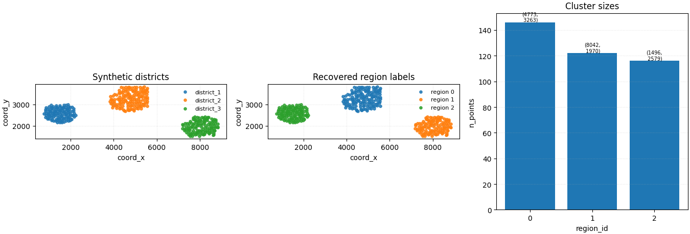
What to learn from this output

The exact integer labels are arbitrary. What matters is the spatial partition they create.

In this lesson, a good result means:

• points that belong to the same compact district mostly share one region label,

• different districts receive different labels,

• the final output is still the full table, only enriched with a new clustering column.

Once a region column exists, it can be reused later for summaries, filtering, diagnostics, or downstream experiments.

Command-line usage

The lesson above used the real CLI entrypoint from Python. At the terminal, the same workflow looks like this:

Basic KMeans clustering with an explicit number of clusters

geoprior-build spatial-clusters \
    cluster_demo_west.csv cluster_demo_east.csv \
    --spatial-cols coord_x coord_y \
    --cluster-col region_id \
    --algorithm kmeans \
    --n-clusters 3 \
    --output cluster_demo_with_regions.csv

The same command through the root dispatcher

geoprior build spatial-clusters \
    cluster_demo_west.csv cluster_demo_east.csv \
    --spatial-cols coord_x coord_y \
    --cluster-col region_id \
    --algorithm kmeans \
    --n-clusters 3 \
    --output cluster_demo_with_regions.csv

Optional diagnostic plot

geoprior-build spatial-clusters \
    cluster_demo_west.csv cluster_demo_east.csv \
    --spatial-cols coord_x coord_y \
    --algorithm kmeans \
    --cluster-col region_id \
    --view \
    --output cluster_demo_with_regions.csv

Other supported backends

geoprior-build spatial-clusters demo.csv \
    --spatial-cols coord_x coord_y \
    --algorithm dbscan \
    --output cluster_demo_dbscan.csv

geoprior-build spatial-clusters demo.csv \
    --spatial-cols coord_x coord_y \
    --algorithm agglo \
    --n-clusters 3 \
    --output cluster_demo_agglo.csv