
Note
Go to the end to download the full example code.
Inspect transfer-learning results before trusting cross-city conclusions#
This lesson explains how to inspect the xfer_results.json artifact.
Unlike most artifacts in the inspection gallery, transfer results are usually stored as a JSON list of records, not as one single mapping. Each record describes one transfer job and combines:
the transfer direction,
the strategy and calibration choices,
overall evaluation metrics,
per-horizon behavior,
schema mismatch diagnostics,
warm-start details,
exported CSV locations.
That makes this artifact especially useful when you want to answer workflow questions such as:
Which transfer direction behaves better?
Does performance collapse as the forecast horizon grows?
Are poor metrics possibly explained by schema mismatch?
Did the warm-start settings look sensible?
Is a cross-city result good enough to compare, report, or extend?
The goal of this page is not only to call plotting helpers. It is to teach how to read transfer results as a comparison artifact and turn that reading into an informed workflow decision.
from __future__ import annotations

import json
import tempfile
from pathlib import Path
from pprint import pprint

import matplotlib.pyplot as plt
import pandas as pd

from geoprior.utils.inspect import (
    generate_xfer_results,
    inspect_xfer_results,
    load_xfer_results,
    plot_xfer_boolean_summary,
    plot_xfer_direction_metric,
    plot_xfer_overall_metrics,
    plot_xfer_per_horizon_metrics,
    plot_xfer_schema_counts,
    summarize_xfer_results,
    xfer_overall_frame,
    xfer_per_horizon_frame,
    xfer_schema_frame,
    xfer_warm_frame,
)

pd.set_option("display.max_columns", 24)
pd.set_option("display.width", 108)

XFER_COLORS = {
    "primary": "#0f766e",
    "secondary": "#2563eb",
    "accent": "#f97316",
    "rose": "#e11d48",
    "gold": "#ca8a04",
    "ink": "#0f172a",
    "muted": "#64748b",
    "grid": "#cbd5e1",
    "face": "#f8fafc",
    "pass": "#16a34a",
    "fail": "#dc2626",
}


def _style_axes(
        ax: plt.Axes, *,
        facecolor: str = XFER_COLORS["face"]
    ) -> None:
    ax.set_facecolor(facecolor)
    ax.set_axisbelow(True)
    ax.grid(
        True,
        color=XFER_COLORS["grid"],
        alpha=0.45,
        linewidth=0.8
    )
    for side in ("top", "right"):
        ax.spines[side].set_visible(False)
    for side in ("left", "bottom"):
        ax.spines[side].set_color("#94a3b8")
        ax.spines[side].set_linewidth(0.9)
    ax.tick_params(colors=XFER_COLORS["ink"], labelsize=9)
    if ax.get_title():
        ax.set_title(
            ax.get_title(),
            fontsize=11,
            fontweight="bold",
             color=XFER_COLORS["ink"],
             pad=12
    )
    if ax.get_xlabel():
        ax.set_xlabel(
            ax.get_xlabel(),
            fontsize=9.5,
            color=XFER_COLORS["muted"]
        )
    if ax.get_ylabel():
        ax.set_ylabel(
            ax.get_ylabel(),
            fontsize=9.5,
            color=XFER_COLORS["muted"]
        )


def _style_bars(
        ax: plt.Axes, colors: list[str], *,
        edgecolor: str = XFER_COLORS["ink"],
        linewidth: float = 1.1,
        alpha: float = 0.94
        ) -> None:
    for idx, patch in enumerate(ax.patches):
        patch.set_facecolor(colors[idx % len(colors)])
        patch.set_edgecolor(edgecolor)
        patch.set_linewidth(linewidth)
        patch.set_alpha(alpha)


def _style_lines(
        ax: plt.Axes, colors: list[str], *,
        markers: tuple[str, ...] = ("o", "s", "D", "^"),
        linewidth: float = 2.4,
        markersize: float = 7.0) -> None:
    for idx, line in enumerate(ax.lines):
        color = colors[idx % len(colors)]
        line.set_color(color)
        line.set_linewidth(linewidth)
        line.set_marker(markers[idx % len(markers)])
        line.set_markersize(markersize)
        line.set_markerfacecolor(color)
        line.set_markeredgecolor("white")
        line.set_markeredgewidth(0.8)


def _style_boolean_bars(ax: plt.Axes) -> None:
    for patch in ax.patches:
        value = patch.get_width() if patch.get_width() else patch.get_height()
        color = XFER_COLORS["pass"] if value >= 0.5 else XFER_COLORS["fail"]
        patch.set_facecolor(color)
        patch.set_edgecolor(XFER_COLORS["ink"])
        patch.set_linewidth(1.1)
        patch.set_alpha(0.95)
Why this artifact matters#
Transfer results are not only about raw accuracy. In a cross-city or cross-domain workflow, a record can look weak for several different reasons:
the transfer direction may be intrinsically harder,
horizon-wise error may grow too quickly,
coverage may be acceptable but intervals may be too wide,
schema mismatch may make the transfer unfair,
warm-start settings may be too small or too aggressive.
Because this file keeps those pieces together, it becomes one of the best places to inspect a transfer experiment before drawing strong scientific or operational conclusions.
Create a realistic demo artifact#
For documentation lessons, we usually want a stable artifact that is rich enough to compare directions without rerunning the full transfer workflow.
Here we generate a small but realistic transfer-results file and make the two directions slightly different on purpose, so the lesson can teach how to interpret comparisons instead of only printing tables.
workdir = Path(tempfile.mkdtemp(prefix="gp_xfer_results_"))
out_dir = workdir
xfer_path = out_dir / "xfer_results.json"

generate_xfer_results(
    xfer_path,
    overrides=[
        {
            "strategy": "warm",
            "calibration": "source",
            "rescale_mode": "strict",
            "coverage80": 0.872,
            "sharpness80": 49.80,
            "overall_mae": 13.90,
            "overall_rmse": 21.75,
            "overall_r2": 0.832,
            "per_horizon_rmse": {
                "H1": 13.90,
                "H2": 20.90,
                "H3": 27.80,
            },
            "schema": {
                "static_missing_n": 7,
                "static_extra_n": 5,
            },
        },
        {
            "strategy": "warm",
            "calibration": "source",
            "rescale_mode": "strict",
            "coverage80": 0.821,
            "sharpness80": 109.20,
            "overall_mae": 37.10,
            "overall_rmse": 61.20,
            "overall_r2": 0.748,
            "per_horizon_rmse": {
                "H1": 18.40,
                "H2": 51.60,
                "H3": 91.50,
            },
            "schema": {
                "static_missing_n": 10,
                "static_extra_n": 12,
            },
        },
    ],
)

print("Written transfer-results file")
print(f" - {xfer_path}")
Written transfer-results file
 - /tmp/gp_xfer_results_db3h6qd7/xfer_results.json
Load the artifact with the real reader#
This artifact family is slightly special: the top-level payload is a list of records rather than a single JSON object. That is already something worth teaching because users often assume every artifact in the workflow has the same shape.
Transfer artifact basics
{'first_record_keys': ['calibration',
                       'coverage80',
                       'csv_eval',
                       'csv_future',
                       'direction',
                       'hps_mode',
                       'job_index',
                       'job_total',
                       'metrics_source',
                       'metrics_unit',
                       'model_dir',
                       'model_name'],
 'n_records': 2,
 'type': 'list'}

First record preview
{
  "strategy": "warm",
  "rescale_mode": "strict",
  "warm": {
    "warm_split": "val",
    "warm_samples": 20000,
    "warm_frac": null,
    "warm_epochs": 3,
    "warm_lr": 0.0001,
    "warm_seed": 42,
    "schema": {
      "src_city": "nansha",
      "tgt_city": "zhongshan",
      "static_aligned": true,
      "dynamic_reordered": false,
      "future_reordered": false,
      "dynamic_order_mismatch": false,
      "future_order_mismatch": false,
      "static_missing_n": 9,
      "static_extra_n": 6
    }
  },
  "model_path": "results/nansha_GeoPriorSubsNet_stage1/train_20260222-141331/nansha_GeoPriorSubsNet_H3_best.keras",
  "split": "test",
  "calibration": "source",
  "quantiles": [
    0.1,
    0.5,
    0.9
  ],
  "coverage80": 0.872,
  "sharpness80": 49.8,
  "overall_mae": 13.9,
  "overall_mse": 499.0390742467,
  "overall_rmse": 21.75,
  "overall_r2": 0.832,
  "per_horizon_mae": {
    "H1": 9.2531121755,
    "H2": 14.4207786362,
    "H3": 19.232098912
  },
  "per_horizon_mse": {
    "H1": 196.9444467984,
    "H2": 465.9660166509,
    "H3": 834.2067592909
  },
  "per_horizon_rmse": {
    "H1": 13.9,
    "H2": 20.9,
    "H3": 27.8
  },
  "per_horizon_r2": {
    "H1": 0.88807
...
Start with the workflow summary#
The compact summary is the quickest way to answer broad questions:
how many transfer jobs are present,
which directions are represented,
which strategies and calibration modes appear,
which record currently looks best by RMSE or R²,
and whether schema mismatch is a recurring pattern.
summary = summarize_xfer_results(records)

print("\nCompact summary")
print(json.dumps(summary, indent=2))
Compact summary
{
  "n_records": 2,
  "directions": [
    "A_to_B",
    "B_to_A"
  ],
  "strategies": [
    "warm"
  ],
  "calibrations": [
    "source"
  ],
  "rescale_modes": [
    "strict"
  ],
  "best_overall_rmse": {
    "label": "A_to_B | warm | source | strict",
    "value": 21.75
  },
  "best_overall_r2": {
    "label": "A_to_B | warm | source | strict",
    "value": 0.832
  },
  "mean_coverage80": 0.8465,
  "mean_sharpness80": 79.5,
  "worst_horizon_rmse": {
    "label": "B_to_A | warm | source | strict",
    "horizon": "H3",
    "value": 91.5
  },
  "schema_pass_rates": {
    "dynamic_order_mismatch": 0.0,
    "dynamic_reordered": 0.0,
    "future_order_mismatch": 0.0,
    "future_reordered": 0.0,
    "static_aligned": 1.0
  },
  "schema_mean_counts": {
    "static_extra_n": 8.5,
    "static_missing_n": 8.5
  }
}
Read the main comparison table#
The overall frame is usually the first table to inspect because it puts the most important workflow columns side by side:
direction,
source and target city,
strategy,
calibration,
rescale mode,
overall quality metrics.
This table is where you normally rank records before drilling into horizon-wise behavior.
overall = xfer_overall_frame(records)

print("\nOverall comparison table")
print(
    overall[
        [
            "label",
            "direction",
            "strategy",
            "calibration",
            "rescale_mode",
            "coverage80",
            "sharpness80",
            "overall_mae",
            "overall_rmse",
            "overall_r2",
        ]
    ]
)

ranked = overall.sort_values("overall_rmse").reset_index(drop=True)
best = ranked.iloc[0]
worst = ranked.iloc[-1]

print("\nInitial reading")
print(
    f"Best overall record by RMSE: {best['label']} "
    f"(RMSE={best['overall_rmse']:.3f}, R²={best['overall_r2']:.3f})."
)
print(
    f"Weakest overall record by RMSE: {worst['label']} "
    f"(RMSE={worst['overall_rmse']:.3f}, R²={worst['overall_r2']:.3f})."
)
Overall comparison table
                             label direction strategy calibration rescale_mode  coverage80  sharpness80  \
0  A_to_B | warm | source | strict    A_to_B     warm      source       strict    0.872000    49.800000
1  B_to_A | warm | source | strict    B_to_A     warm      source       strict    0.821000   109.200000

   overall_mae  overall_rmse  overall_r2
0    13.900000     21.750000    0.832000
1    37.100000     61.200000    0.748000

Initial reading
Best overall record by RMSE: A_to_B | warm | source | strict (RMSE=21.750, R²=0.832).
Weakest overall record by RMSE: B_to_A | warm | source | strict (RMSE=61.200, R²=0.748).
Interpret overall metrics carefully#
In transfer settings, no single metric is enough.
A practical reading habit is:
look at RMSE or MAE for error magnitude,
look at R² for explained variation,
look at coverage80 to see whether intervals are too narrow,
look at sharpness80 to see whether acceptable coverage was paid for with very wide intervals.
This last point is especially important in transfer workflows: wide intervals can make a model look safer than it really is.
coverage_gap = float(best["coverage80"] - worst["coverage80"])
sharpness_gap = float(worst["sharpness80"] - best["sharpness80"])

print("\nCoverage / sharpness reading")
print(
    f"Coverage difference between strongest and weakest record: "
    f"{coverage_gap:.3f}."
)
print(
    f"Sharpness penalty of the weaker record relative to the stronger one: "
    f"{sharpness_gap:.3f}."
)
Coverage / sharpness reading
Coverage difference between strongest and weakest record: 0.051.
Sharpness penalty of the weaker record relative to the stronger one: 59.400.
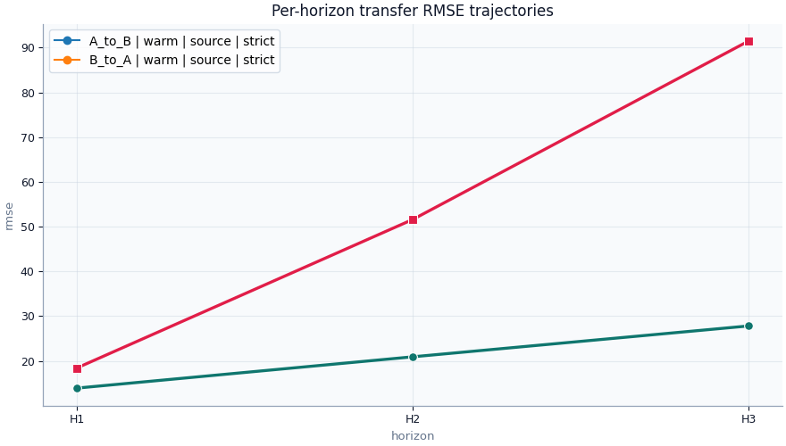
Inspect per-horizon degradation#
Transfer experiments often look acceptable overall while hiding a severe collapse at the farthest horizon. That is why the per-horizon frame is one of the most important views in this artifact family.
We focus on RMSE here because it is easy to compare across directions, but the same table also contains MAE, MSE, and R².
per_h = xfer_per_horizon_frame(records)

print("\nPer-horizon comparison (RMSE only)")
print(
    per_h.loc[
        per_h["metric"] == "rmse",
        ["label", "direction", "horizon", "value"],
    ]
)

rmse_h = per_h[per_h["metric"] == "rmse"].copy()
horizon_spread = (
    rmse_h.groupby("label")["value"].agg(["min", "max"])
    .assign(range=lambda d: d["max"] - d["min"])
    .sort_values("range", ascending=False)
)

print("\nHorizon spread in RMSE")
print(horizon_spread)

print(
    "\nInterpretation:\n"
    "A large RMSE range across H1→H3 usually means the transfer is\n"
    "less reliable for longer horizons, even if the overall metric\n"
    "still looks acceptable."
)
Per-horizon comparison (RMSE only)
                              label direction horizon     value
18  A_to_B | warm | source | strict    A_to_B      H1 13.900000
19  A_to_B | warm | source | strict    A_to_B      H2 20.900000
20  A_to_B | warm | source | strict    A_to_B      H3 27.800000
21  B_to_A | warm | source | strict    B_to_A      H1 18.400000
22  B_to_A | warm | source | strict    B_to_A      H2 51.600000
23  B_to_A | warm | source | strict    B_to_A      H3 91.500000

Horizon spread in RMSE
                                      min       max     range
label
B_to_A | warm | source | strict 18.400000 91.500000 73.100000
A_to_B | warm | source | strict 13.900000 27.800000 13.900000

Interpretation:
A large RMSE range across H1→H3 usually means the transfer is
less reliable for longer horizons, even if the overall metric
still looks acceptable.
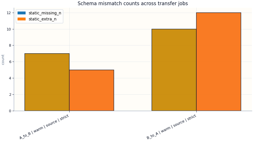
Inspect schema mismatch diagnostics#
One of the most helpful parts of this artifact is that it keeps schema alignment diagnostics next to the metrics. This is very useful when comparing cities with different static-feature support.
A poor transfer result does not automatically mean the learning strategy failed. It may partly reflect missing or extra feature channels between source and target.
schema = xfer_schema_frame(records)

print("\nSchema diagnostics")
print(schema)

schema_counts = schema[schema["kind"] == "count"].copy()
if not schema_counts.empty:
    schema_pivot = schema_counts.pivot(
        index="label",
        columns="name",
        values="value",
    ).fillna(0.0)
    print("\nSchema mismatch count table")
    print(schema_pivot)
Schema diagnostics
                              label direction source_city target_city strategy   kind  \
0   A_to_B | warm | source | strict    A_to_B      nansha   zhongshan     warm   bool
1   A_to_B | warm | source | strict    A_to_B      nansha   zhongshan     warm   bool
2   A_to_B | warm | source | strict    A_to_B      nansha   zhongshan     warm   bool
3   A_to_B | warm | source | strict    A_to_B      nansha   zhongshan     warm   bool
4   A_to_B | warm | source | strict    A_to_B      nansha   zhongshan     warm   bool
5   A_to_B | warm | source | strict    A_to_B      nansha   zhongshan     warm  count
6   A_to_B | warm | source | strict    A_to_B      nansha   zhongshan     warm  count
7   B_to_A | warm | source | strict    B_to_A   zhongshan      nansha     warm   bool
8   B_to_A | warm | source | strict    B_to_A   zhongshan      nansha     warm   bool
9   B_to_A | warm | source | strict    B_to_A   zhongshan      nansha     warm   bool
10  B_to_A | warm | source | strict    B_to_A   zhongshan      nansha     warm   bool
11  B_to_A | warm | source | strict    B_to_A   zhongshan      nansha     warm   bool
12  B_to_A | warm | source | strict    B_to_A   zhongshan      nansha     warm  count
13  B_to_A | warm | source | strict    B_to_A   zhongshan      nansha     warm  count

                      name     value
0           static_aligned      True
1        dynamic_reordered     False
2         future_reordered     False
3   dynamic_order_mismatch     False
4    future_order_mismatch     False
5         static_missing_n  7.000000
6           static_extra_n  5.000000
7           static_aligned      True
8        dynamic_reordered     False
9         future_reordered     False
10  dynamic_order_mismatch     False
11   future_order_mismatch     False
12        static_missing_n 10.000000
13          static_extra_n 12.000000

Schema mismatch count table
name                            static_extra_n static_missing_n
label
A_to_B | warm | source | strict       5.000000         7.000000
B_to_A | warm | source | strict      12.000000        10.000000
Inspect warm-start details#
The warm-start frame is useful for reproducibility. When two runs are compared, we should confirm they were warmed under comparable settings before attributing differences entirely to city direction or schema quality.
Warm-start settings
                             label direction strategy warm_split  warm_samples warm_frac  warm_epochs  \
0  A_to_B | warm | source | strict    A_to_B     warm        val  20000.000000      None     3.000000
1  B_to_A | warm | source | strict    B_to_A     warm        val  20000.000000      None     3.000000

   warm_lr  warm_seed
0 0.000100  42.000000
1 0.000100  42.000000
Use the all-in-one inspector when you want all core views together#
inspect_xfer_results(...) is convenient when you want the
semantic summary plus the main comparison tables returned in one
normalized bundle.
Inspector bundle keys
['overall', 'per_horizon', 'schema', 'summary', 'warm']
Plot the main comparison views#
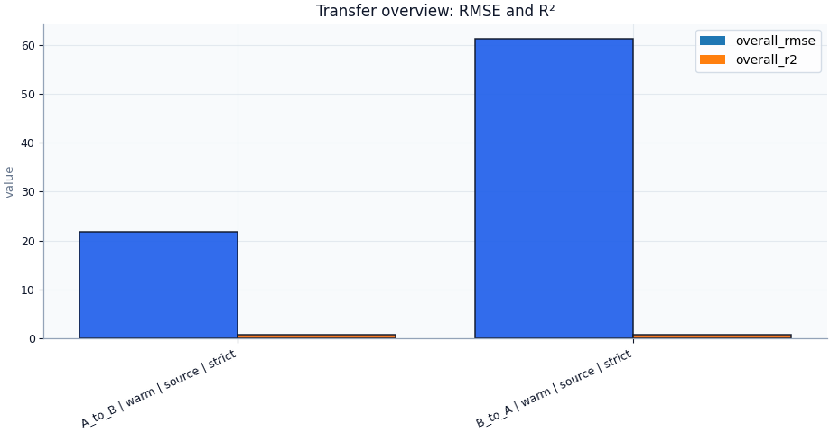
A compact reading session usually benefits from four visuals:
overall metrics for each record,
one direct direction comparison,
per-horizon RMSE trajectories,
schema mismatch counts.
Together, these answer the most common question in transfer work: Which direction looks better, and why?
fig, ax = plot_xfer_overall_metrics(
records,
metrics=["overall_rmse", "overall_r2"],
figsize=(9.2, 4.8),
)
_style_axes(ax, facecolor="#f8fafc")
_style_bars(
ax,
[
XFER_COLORS["secondary"],
XFER_COLORS["secondary"],
XFER_COLORS["accent"],
XFER_COLORS["accent"],
],
)
ax.set_title("Transfer overview: RMSE and R²")
if ax.get_legend() is not None:
ax.get_legend().get_frame().set_facecolor("white")
ax.get_legend().get_frame().set_edgecolor("#cbd5e1")
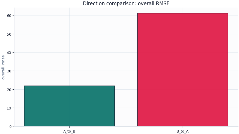
fig, ax = plot_xfer_direction_metric(
records,
metric="overall_rmse",
figsize=(8.2, 4.6),
)
_style_axes(ax, facecolor="#fcfcfd")
_style_bars(ax, [XFER_COLORS["primary"], XFER_COLORS["rose"]])
ax.set_title("Direction comparison: overall RMSE")
fig, ax = plot_xfer_per_horizon_metrics(
records,
metric="rmse",
figsize=(8.8, 5.0),
)
_style_axes(ax, facecolor="#f8fafc")
_style_lines(ax, [XFER_COLORS["primary"], XFER_COLORS["rose"]])
ax.set_title("Per-horizon transfer RMSE trajectories")
if ax.get_legend() is not None:
ax.get_legend().get_frame().set_facecolor("white")
ax.get_legend().get_frame().set_edgecolor("#cbd5e1")
fig, ax = plot_xfer_schema_counts(records, figsize=(8.8, 4.9))
_style_axes(ax, facecolor="#fffdf8")
_style_bars(
ax,
[
XFER_COLORS["gold"],
XFER_COLORS["gold"],
XFER_COLORS["accent"],
XFER_COLORS["accent"],
],
)
ax.set_title("Schema mismatch counts across transfer jobs")
if ax.get_legend() is not None:
ax.get_legend().get_frame().set_facecolor("white")
ax.get_legend().get_frame().set_edgecolor("#cbd5e1")
How to read these plots#
A practical interpretation pattern is:
If one direction is better on overall RMSE and keeps a flatter per-horizon error curve, it is usually the stronger transfer.
If two directions look similar in metrics but one has far fewer schema mismatches, that direction is usually easier to trust.
If coverage is decent only because sharpness is extremely large, the intervals may be too conservative to be useful.
If H3 error grows sharply while H1 looks fine, the model may be acceptable for short-horizon adaptation but not for longer-horizon forecasting.
Plot the boolean summary separately#
The boolean summary aggregates the schema pass/fail checks into one compact view. It is not a performance plot; it is a structural plausibility check for the transfer setup.
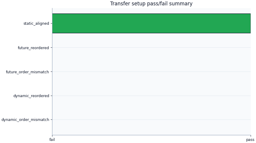
Text(0.5, 1.0, 'Transfer setup pass/fail summary')
A simple decision rule#
For transfer results, a pragmatic reading rule can be:
prefer the direction with the lower overall RMSE,
check that its farthest-horizon RMSE does not explode,
prefer runs with smaller schema mismatch counts,
and be cautious when sharpness becomes very large relative to the better direction.
This is not a theorem. It is a good workflow habit for deciding whether a cross-city result is ready for reporting or whether it still needs schema cleanup, rescaling changes, or a different transfer strategy.
winner = ranked.iloc[0]
loser = ranked.iloc[-1]

winner_schema = schema_counts[
    schema_counts["label"] == winner["label"]
]["value"].sum()
loser_schema = schema_counts[
    schema_counts["label"] == loser["label"]
]["value"].sum()

winner_h3 = rmse_h[
    (rmse_h["label"] == winner["label"])
    & (rmse_h["horizon"] == "H3")
]["value"]
winner_h3 = float(winner_h3.iloc[0]) if not winner_h3.empty else None

print("\nDecision note")
if (
    float(winner["overall_rmse"]) < float(loser["overall_rmse"])
    and float(winner["sharpness80"]) <= float(loser["sharpness80"])
    and float(winner_schema) <= float(loser_schema)
):
    print(
        "The stronger direction in this demo looks structurally and "
        "numerically preferable for follow-up transfer analysis."
    )
else:
    print(
        "The transfer comparison still looks ambiguous and deserves "
        "closer schema or calibration review before reporting."
    )

if winner_h3 is not None:
    print(
        f"The preferred direction still reaches H3 RMSE={winner_h3:.3f}; "
        "decide whether that is acceptable for your scientific or "
        "operational horizon."
    )
Decision note
The stronger direction in this demo looks structurally and numerically preferable for follow-up transfer analysis.
The preferred direction still reaches H3 RMSE=27.800; decide whether that is acceptable for your scientific or operational horizon.
Total running time of the script: (0 minutes 0.563 seconds)