Create district grid layers from forecast points

This example teaches you how to use GeoPrior’s make-district-grid utility.

Unlike the plotting scripts, this command builds a reusable spatial layer. It turns forecast point locations into a regular grid of named zones, optionally clipped to a city boundary.

Why this matters

Later workflows often need a simple district-like support layer for:

• aggregating hotspot statistics,

• assigning samples to zones,

• tagging clusters with zone IDs,

• and producing map-ready spatial summaries.

This builder creates exactly that layer from the forecast point cloud.

Imports

We call the real production entrypoint from the project code. Then we read the generated grid back in and build one compact teaching preview.

from __future__ import annotations

import tempfile
from pathlib import Path

import geopandas as gpd
import matplotlib.pyplot as plt
import numpy as np
import pandas as pd
from shapely.geometry import Polygon

from geoprior.scripts.make_district_grid import (
    make_district_grid_main,
)
from geoprior.scripts import utils as script_utils

Build compact synthetic point clouds

The production script only needs:

• sample_idx

• coord_x

• coord_y

in both eval and future CSVs.

For the lesson, we create two cities with slightly different spatial footprints and one future cloud that extends a bit beyond the eval cloud.

rng = np.random.default_rng(13)


def _city_points(
    *,
    city: str,
    center_x: float,
    center_y: float,
    scale_x: float,
    scale_y: float,
    drift_x: float,
    drift_y: float,
    n: int = 140,
) -> tuple[pd.DataFrame, pd.DataFrame]:
    ang = rng.uniform(0.0, 2.0 * np.pi, size=n)
    rad = np.sqrt(rng.uniform(0.0, 1.0, size=n))

    xe = center_x + scale_x * rad * np.cos(ang)
    ye = center_y + scale_y * rad * np.sin(ang)

    xf = (
        center_x
        + drift_x
        + 1.08 * scale_x * rad * np.cos(ang)
        + rng.normal(0.0, 2.5, size=n)
    )
    yf = (
        center_y
        + drift_y
        + 1.08 * scale_y * rad * np.sin(ang)
        + rng.normal(0.0, 2.0, size=n)
    )

    eval_df = pd.DataFrame(
        {
            "city": city,
            "sample_idx": np.arange(n, dtype=int),
            "coord_x": xe.astype(float),
            "coord_y": ye.astype(float),
        }
    )

    future_df = pd.DataFrame(
        {
            "city": city,
            "sample_idx": np.arange(n, dtype=int),
            "coord_x": xf.astype(float),
            "coord_y": yf.astype(float),
        }
    )

    return eval_df, future_df


ns_eval_df, ns_future_df = _city_points(
    city="Nansha",
    center_x=1200.0,
    center_y=780.0,
    scale_x=120.0,
    scale_y=80.0,
    drift_x=18.0,
    drift_y=8.0,
)

zh_eval_df, zh_future_df = _city_points(
    city="Zhongshan",
    center_x=1720.0,
    center_y=1080.0,
    scale_x=160.0,
    scale_y=95.0,
    drift_x=26.0,
    drift_y=12.0,
)

print("Nansha eval preview")
print(ns_eval_df.head(6).to_string(index=False))

print("")
print("Zhongshan future preview")
print(zh_future_df.head(6).to_string(index=False))

Nansha eval preview
  city  sample_idx   coord_x  coord_y
Nansha           0 1242.2893 747.9394
Nansha           1 1251.9537 735.5226
Nansha           2 1215.4520 754.4628
Nansha           3 1194.4141 831.6899
Nansha           4 1253.9047 798.9406
Nansha           5 1220.1420 775.3049

Zhongshan future preview
     city  sample_idx   coord_x   coord_y
Zhongshan           0 1840.4567 1031.2511
Zhongshan           1 1780.8321 1035.0501
Zhongshan           2 1669.2895 1168.7990
Zhongshan           3 1762.6498 1100.6061
Zhongshan           4 1652.3113 1043.7889
Zhongshan           5 1791.8844 1185.6534

Write the lesson inputs

We follow the real command’s file-based workflow with explicit per-city eval/future CSVs.

tmp_dir = Path(
    tempfile.mkdtemp(prefix="gp_sg_district_grid_")
)

ns_eval_csv = tmp_dir / "nansha_eval.csv"
ns_future_csv = tmp_dir / "nansha_future.csv"
zh_eval_csv = tmp_dir / "zhongshan_eval.csv"
zh_future_csv = tmp_dir / "zhongshan_future.csv"

ns_eval_df.to_csv(ns_eval_csv, index=False)
ns_future_df.to_csv(ns_future_csv, index=False)
zh_eval_df.to_csv(zh_eval_csv, index=False)
zh_future_df.to_csv(zh_future_csv, index=False)

print("")
print("Input files")
for p in [
    ns_eval_csv,
    ns_future_csv,
    zh_eval_csv,
    zh_future_csv,
]:
    print(" -", p.name)

Input files
 - nansha_eval.csv
 - nansha_future.csv
 - zhongshan_eval.csv
 - zhongshan_future.csv

Build a simple boundary file for clipping

The production script accepts an optional boundary GeoJSON/SHP. To make the lesson concrete, we provide one here so the page can show boundary clipping and sample assignment together.

A single dissolved geometry is enough because the script unions the boundary internally.

boundary_poly = Polygon(
    [
        (1070.0, 700.0),
        (1355.0, 710.0),
        (1385.0, 835.0),
        (1260.0, 900.0),
        (1100.0, 870.0),
        (1055.0, 760.0),
    ]
)

boundary_gdf = gpd.GeoDataFrame(
    {"name": ["lesson_boundary"]},
    geometry=[boundary_poly],
    crs=None,
)

boundary_geojson = tmp_dir / "lesson_boundary.geojson"
boundary_gdf.to_file(boundary_geojson, driver="GeoJSON")

print("")
print(f"Boundary file: {boundary_geojson.name}")

Boundary file: lesson_boundary.geojson

Run the real district-grid builder

We ask the production command to:

• use only Nansha for this compact example,

• build a 6 x 5 grid,

• clip it to the boundary,

• write GeoJSON,

• and also emit sample-to-zone assignments.

out_stem = "district_grid_gallery"

make_district_grid_main(
    [
        "--cities", "ns",
        "--ns-eval",
        str(ns_eval_csv),
        "--ns-future",
        str(ns_future_csv),
        "--nx",
        "6",
        "--ny",
        "5",
        "--pad",
        "0.03",
        "--boundary",
        str(boundary_geojson),
        "--clip-boundary",
        "--min-area-frac",
        "0.03",
        "--format",
        "geojson",
        "--assign-samples",
        "--out",
        str(tmp_dir / out_stem),
    ],
    prog="make-district-grid",
)

[OK] wrote /tmp/gp_sg_district_grid_77qhhlt5/district_grid_gallery_nansha.geojson
[OK] wrote /tmp/gp_sg_district_grid_77qhhlt5/district_assignments_nansha.csv

Inspect the produced artifacts

In grid mode the command writes:

• one city-specific grid file,

• and, when requested, one city-specific assignment CSV.

written = sorted(tmp_dir.glob("district_grid_gallery*"))
assignments = sorted(tmp_dir.glob("district_assignments_*.csv"))

print("")
print("Written files")
for p in written + assignments:
    print(" -", p.name)

Written files
 - district_grid_gallery_nansha.geojson
 - district_assignments_nansha.csv

Read the generated outputs

We read both the grid layer and the assignment table back in.

grid_geojson = tmp_dir / "district_grid_gallery_nansha.geojson"
assign_csv = tmp_dir / "district_assignments_nansha.csv"

grid_gdf = gpd.read_file(grid_geojson)
assign_df = pd.read_csv(assign_csv)

print("")
print("Grid preview")
print(
    grid_gdf[
        [
            "city",
            "zone_id",
            "zone_label",
            "row",
            "col",
            "xmin",
            "xmax",
            "ymin",
            "ymax",
        ]
    ].head(10).to_string(index=False)
)

print("")
print("Assignments preview")
print(assign_df.head(10).to_string(index=False))

Grid preview
  city zone_id zone_label  row  col      xmin      xmax     ymin     ymax
Nansha   Z0501 Zone Z0501    4    0 1077.6938 1119.2035 697.0625 729.2833
Nansha   Z0502 Zone Z0502    4    1 1119.2035 1160.7132 697.0625 729.2833
Nansha   Z0503 Zone Z0503    4    2 1160.7132 1202.2229 697.0625 729.2833
Nansha   Z0504 Zone Z0504    4    3 1202.2229 1243.7326 697.0625 729.2833
Nansha   Z0505 Zone Z0505    4    4 1243.7326 1285.2423 697.0625 729.2833
Nansha   Z0506 Zone Z0506    4    5 1285.2423 1326.7520 697.0625 729.2833
Nansha   Z0401 Zone Z0401    3    0 1077.6938 1119.2035 729.2833 761.5041
Nansha   Z0402 Zone Z0402    3    1 1119.2035 1160.7132 729.2833 761.5041
Nansha   Z0403 Zone Z0403    3    2 1160.7132 1202.2229 729.2833 761.5041
Nansha   Z0404 Zone Z0404    3    3 1202.2229 1243.7326 729.2833 761.5041

Assignments preview
  city  sample_idx   coord_x  coord_y zone_id  zone_row  zone_col  zone_present
Nansha           0 1242.2893 747.9394   Z0404         3         3          True
Nansha           1 1251.9537 735.5226   Z0405         3         4          True
Nansha           2 1215.4520 754.4628   Z0404         3         3          True
Nansha           3 1194.4141 831.6899   Z0103         0         2          True
Nansha           4 1253.9047 798.9406   Z0205         1         4          True
Nansha           5 1220.1420 775.3049   Z0304         2         3          True
Nansha           6 1151.1024 751.6976   Z0402         3         1          True
Nansha           7 1315.6076 781.2741   Z0306         2         5          True
Nansha           8 1273.9309 748.8980   Z0405         3         4          True
Nansha           9 1262.5112 776.0087   Z0305         2         4          True

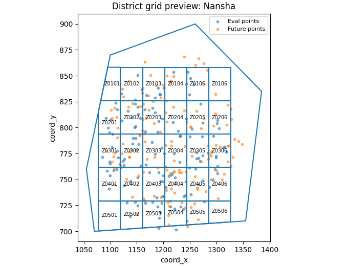
Build one compact visual preview

This preview is not part of the production builder itself. It is a teaching aid for the gallery page.

It overlays:

• eval and future points,

• the boundary,

• the clipped district grid.

fig, ax = plt.subplots(
    figsize=(6.8, 5.2),
    constrained_layout=True,
)

ax.scatter(
    ns_eval_df["coord_x"].to_numpy(float),
    ns_eval_df["coord_y"].to_numpy(float),
    s=10,
    alpha=0.55,
    label="Eval points",
)
ax.scatter(
    ns_future_df["coord_x"].to_numpy(float),
    ns_future_df["coord_y"].to_numpy(float),
    s=10,
    alpha=0.55,
    label="Future points",
)

boundary_gdf.boundary.plot(ax=ax)
grid_gdf.boundary.plot(ax=ax)

for _, row in grid_gdf.iterrows():
    rp = row.geometry.representative_point()
    ax.text(
        rp.x,
        rp.y,
        str(row["zone_id"]),
        ha="center",
        va="center",
        fontsize=7,
    )

ax.set_title("District grid preview: Nansha")
ax.set_xlabel("coord_x")
ax.set_ylabel("coord_y")
ax.legend(fontsize=8)

<matplotlib.legend.Legend object at 0x749e56c0b9b0>

Learn how to read the grid artifact

Each grid row represents one zone polygon with:

• zone_id: a compact ID such as Z0305,

• row: north-to-south row index starting at 0,

• col: west-to-east column index starting at 0,

• bounding coordinates,

• and geometry.

The geometry is the full cell unless boundary clipping is enabled.

Learn how the zone IDs are formed

The script numbers rows from the north (top) downward and columns from the west (left) eastward.

So:

• Z0101 is the north-west corner,

• Z0201 is one row farther south,

• Z0102 is one column farther east.

This is useful because the IDs remain stable and readable even after clipping.

Why clipping matters

Without a boundary, the builder creates a full rectangular grid over the padded point extent.

With --clip-boundary, each cell is intersected with the boundary polygon, and tiny slivers can be dropped using --min-area-frac.

That makes the final grid much more suitable for map overlays or zone-based reporting.

Why the assignment CSV is useful

With --assign-samples, the script also writes a compact table mapping each sample point to:

• zone_id

• zone_row

• zone_col

and, when clipping was used, a zone_present flag telling you whether that assigned zone survived clipping.

This is especially handy for later scripts that tag clusters or aggregate point-level outputs by zone.

Why this page belongs after make_boundary.py

The natural workflow is:

1. build a boundary,

2. build a district grid over the city footprint,

3. optionally assign samples to grid zones,

4. reuse the zones in exposure or cluster-tagging steps.

So this page is best seen as the next support-layer lesson after the boundary page.

Command-line version

The same lesson can be reproduced from the CLI.

Legacy dispatcher:

python -m scripts make-district-grid \
  --ns-eval results/nansha_eval.csv \
  --ns-future results/nansha_future.csv \
  --nx 12 \
  --ny 12 \
  --boundary boundary_nansha.geojson \
  --clip-boundary \
  --assign-samples \
  --format both \
  --out district_grid

Modern CLI:

geoprior build district-grid \
  --ns-eval results/nansha_eval.csv \
  --ns-future results/nansha_future.csv \
  --nx 12 \
  --ny 12 \
  --boundary boundary_nansha.geojson \
  --clip-boundary \
  --assign-samples \
  --format both \
  --out district_grid

Source-folder discovery:

geoprior build district-grid \
  --ns-src results/nansha_run \
  --zh-src results/zhongshan_run \
  --split auto \
  --nx 12 \
  --ny 12 \
  --pad 0.02 \
  --format geojson \
  --out district_grid

The gallery page teaches the builder. The command line reproduces it in a workflow.