Applications#

This gallery presents GeoPrior as a scientific workflow rather than as an isolated model or a collection of figures. Each page starts from a practical question, builds the relevant evidence, and then shows how the result can support interpretation, auditing, external anchoring, intervention planning, or cross-city deployment.

Why this gallery matters#

In geohazard forecasting, good metrics alone are not enough. A model may fit the data while remaining hard to trust, difficult to interpret, only partially anchored to field evidence, or poorly suited to deployment in a new basin. The pages collected here are therefore organized around five higher-level questions:

Does the physics-guided model create measurable value?
Can the learned physical fields be interpreted responsibly?
Are the inferred effective pathways anchored to independent site evidence?
How do probabilistic forecasts become intervention priorities?
How much skill survives when the workflow is transferred to a new city?

Taken together, these applications show how GeoPrior supports a full reasoning chain from predictive skill to interpretability, field anchoring, decision support, and cross-city rollout.

How to read the gallery#

A good reading order is the one below.

Step	Page	Why start here
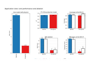
Core value	`app_core_ablation.py`	Start here to see what the physics-guided pathway changes in practice. This page compares the with-physics and no-physics variants under the same data pathway and training setup, so the reader can isolate what the physical scaffold contributes to accuracy, calibration, and interval usefulness.
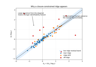
Interpretation guardrails	`app_bounds_ridge.py`	Continue here to audit identifiability. This page explains why effective timescales can be more robust than a literal decomposition into \(K\), \(S_s\), and \(H_d\), and why ridge and bounds diagnostics are necessary before turning learned fields into physical claims.
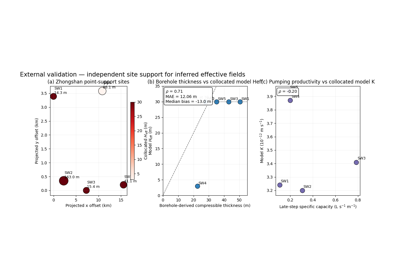
Field anchoring	`app_external_validation.py`	Read this page when the question shifts from internal coherence to external support. It shows how independent borehole and pumping-test information can anchor the thickness pathway, while also clarifying which parts of the inferred physics remain only weakly constrained.
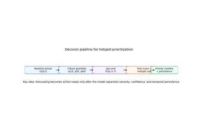
Action prioritization	`app_hotspot_prioritization.py`	Move here when the question is not only where subsidence is forecast, but where action should begin. This page turns calibrated forecast quantiles into exceedance maps, hotspot clusters, persistence summaries, and ranked intervention targets.
Cross-city rollout	`app_transferability.py`	Finish here to understand deployment beyond the training city. This page compares baseline, zero-shot transfer, and warm-start adaptation through retained point skill, uncertainty quality, threshold-risk behavior, and hotspot stability.

What these pages emphasize#

These application lessons are designed to answer five distinct kinds of scientific and operational questions.

Validation: app_core_ablation.py demonstrates whether the physics-aware scaffold produces tangible forecasting value instead of acting as a decorative regularizer.
Auditability: app_bounds_ridge.py shows how GeoPrior can critique its own inferred fields by exposing clipping, ridge structure, and the limits of direct parameter interpretation.
Field anchoring: app_external_validation.py shows how independent site evidence can support the thickness pathway while also clarifying the limits of sparse field checks for conductivity-like quantities.
Decision support: app_hotspot_prioritization.py shows how uncertainty-aware forecasts become practical spatial priorities rather than ending as static forecast maps.
Deployment realism: app_transferability.py shows what survives distribution shift, what degrades under zero-shot reuse, and how adaptation restores usable skill.

Common pattern across the applications#

Although each page addresses a different objective, they all follow the same broad structure:

a concrete applied question,
a short scientific motivation,
one main figure or analytic view,
one or more supporting diagnostics,
an interpretation section that clarifies what can be concluded safely,
and a reproducible path back to the scripts and exported tables.

This is intentional. The goal is to make the gallery useful to several kinds of readers at once: researchers evaluating the method, practitioners looking for operational outputs, and developers who want a clear path from raw artifacts to interpretable products.

Where to go next#

After reading these applications, the rest of the example gallery can be used more surgically:

the forecasting pages for horizon-by-horizon forecast behavior,
the uncertainty pages for calibration and interval diagnostics,
the diagnostics pages for training, tuning, and physics checks,
and the figure_generation pages for the lower-level plots used to build the application narratives.

In that sense, the application gallery is the synthesis layer: it does not replace the rest of the examples, but shows how those building blocks come together in a coherent scientific workflow.

Auditing identifiability before reading learned physics fields

Why physics matters in core forecasting

External validation of inferred effective fields

From calibrated forecasts to action-first zones

When cross-city reuse is useful, and when it is not