
Note
Go to the end to download the full example code.
Inspect ablation records before choosing a configuration#
This lesson explains how to inspect the JSONL artifact
ablation_record.jsonl.
Why this file matters#
Ablation work is not only about finding the best score. It is about understanding why one configuration behaves differently from another. In practice, an ablation record helps answer questions such as:
Which variant really reduced RMSE or MAE?
Was the apparent gain only at short horizons?
Did a physics-weight change improve fit while harming stability?
Are two variants actually comparable in their lambda weights?
Is a strong score still believable when epsilon diagnostics degrade?
This page is therefore written as a reading lesson, not only as an API demo. We will use the ablation inspector to move from raw JSONL records to interpretable tables, comparison plots, and a final decision rule.
from __future__ import annotations

import json
import tempfile
from pathlib import Path
from pprint import pprint

import matplotlib.pyplot as plt
import pandas as pd

from geoprior.utils.inspect import (
    ablation_config_frame,
    ablation_metrics_frame,
    ablation_per_horizon_frame,
    ablation_record_flags_frame,
    ablation_record_runs_frame,
    generate_ablation_record,
    inspect_ablation_record,
    load_ablation_record,
    plot_ablation_boolean_summary,
    plot_ablation_lambda_weights,
    plot_ablation_metric_by_variant,
    plot_ablation_per_horizon_metric,
    plot_ablation_run_counts,
    plot_ablation_top_variants,
    summarize_ablation_record,
)

pd.set_option("display.max_columns", 32)
pd.set_option("display.width", 110)
pd.set_option("display.float_format", lambda v: f"{v:0.6f}")

ABLATION_PALETTE = {
    "counts": ["#4C78A8", "#72B7B2", "#54A24B", "#F58518"],
    "rmse": ["#2E86AB", "#A23B72", "#F18F01", "#C73E1D"],
    "lambdas": ["#355070", "#6D597A", "#B56576", "#E56B6F", "#EAAC8B", "#84A59D", "#52796F"],
    "horizon_lines": ["#3A86FF", "#8338EC", "#FF006E", "#FB5607"],
    "top": ["#118AB2", "#06D6A0", "#FFD166", "#EF476F"],
    "checks": "#5C677D",
}
JSONL is a little different from the other artifacts#
Most inspection files in this gallery are single JSON objects.
ablation_record.jsonl is different: it is a newline-delimited log,
so each line is one ablation record.
That difference matters conceptually:
we are usually comparing variants, not reading one run in isolation,
there may be multiple seeds or repeated evaluations,
one metric alone is rarely enough to choose a variant.
In other words, the goal is to compare patterns across records.
Create a realistic demo ablation file#
For a gallery lesson, we want a stable and readable set of ablation rows without rerunning the full experiment pipeline.
The helper already creates a realistic family of records, but here we push the variants a little further apart so the lesson becomes easier to interpret:
baselinestays as the reference,gw_heaviergets a larger groundwater weight,smoothermakes the smoothness term more visible,bounds_strongerincreases the bounds penalty.
This is a good teaching setup because it gives us meaningful differences in both scalar and horizon-wise behavior.
workdir = Path(tempfile.mkdtemp(prefix="gp_ablation_"))
out_dir = workdir
ablation_path = out_dir / "nansha_ablation_record.jsonl"

generate_ablation_record(
    ablation_path,
    overrides=[
        {
            "ablation": "baseline",
            "seed": 11,
            "lambda_gw": 0.10,
            "lambda_smooth": 0.010,
            "lambda_bounds": 0.05,
            "mae": 0.01190,
            "rmse": 0.01776,
            "r2": 0.87970,
            "epsilon_prior": 8.78,
            "per_horizon_mae": {
                "H1": 0.00536,
                "H2": 0.01229,
                "H3": 0.01807,
            },
            "per_horizon_r2": {
                "H1": 0.8924,
                "H2": 0.8812,
                "H3": 0.8720,
            },
        },
        {
            "ablation": "gw_heavier",
            "seed": 12,
            "lambda_gw": 0.18,
            "lambda_smooth": 0.010,
            "lambda_bounds": 0.05,
            "mae": 0.01135,
            "rmse": 0.01710,
            "r2": 0.88450,
            "epsilon_prior": 9.35,
            "per_horizon_mae": {
                "H1": 0.00510,
                "H2": 0.01166,
                "H3": 0.01729,
            },
            "per_horizon_r2": {
                "H1": 0.8960,
                "H2": 0.8865,
                "H3": 0.8758,
            },
        },
        {
            "ablation": "smoother",
            "seed": 13,
            "lambda_gw": 0.10,
            "lambda_smooth": 0.050,
            "lambda_bounds": 0.05,
            "mae": 0.01225,
            "rmse": 0.01802,
            "r2": 0.87720,
            "epsilon_prior": 7.95,
            "per_horizon_mae": {
                "H1": 0.00562,
                "H2": 0.01256,
                "H3": 0.01857,
            },
            "per_horizon_r2": {
                "H1": 0.8910,
                "H2": 0.8790,
                "H3": 0.8680,
            },
        },
        {
            "ablation": "bounds_stronger",
            "seed": 14,
            "lambda_gw": 0.10,
            "lambda_smooth": 0.010,
            "lambda_bounds": 0.12,
            "mae": 0.01170,
            "rmse": 0.01742,
            "r2": 0.88210,
            "epsilon_prior": 8.12,
            "per_horizon_mae": {
                "H1": 0.00518,
                "H2": 0.01202,
                "H3": 0.01796,
            },
            "per_horizon_r2": {
                "H1": 0.8948,
                "H2": 0.8832,
                "H3": 0.8731,
            },
        },
    ],
)

print("Written ablation file")
print(f" - {ablation_path}")
Written ablation file
 - /tmp/gp_ablation_nxwhtrru/nansha_ablation_record.jsonl
Look at the raw JSONL form first#
Before using the inspection helpers, it is useful to remember what this artifact really looks like on disk. Each line is its own JSON record. This is one reason why the ablation inspector uses tables so heavily: raw JSONL becomes hard to compare once the file grows.
print("\nFirst two raw lines")
with ablation_path.open("r", encoding="utf-8") as stream:
    for idx, line in enumerate(stream, start=1):
        print(line.strip())
        if idx >= 2:
            break
First two raw lines
{"timestamp": "20260228-191355", "city": "nansha", "model": "GeoPriorSubsNet", "pde_mode": "both", "use_effective_h": true, "kappa_mode": "kb", "hd_factor": 0.6, "lambda_cons": 0.0, "lambda_gw": 0.1, "lambda_prior": 0.0, "lambda_smooth": 0.01, "lambda_mv": 0.0, "lambda_bounds": 0.05, "lambda_q": 0.0005, "r2": 0.8797, "mse": 0.000315, "mae": 0.0119, "rmse": 0.01776, "coverage80": 0.8554, "sharpness80": 0.0454, "metrics": {"r2": 0.8797, "mse": 0.000315, "mae": 0.0119, "rmse": 0.0178, "coverage80": 0.8554, "sharpness80": 0.0454, "units": {"subs_unit_to_si": 0.001, "subs_factor_si_to_real": 1000.0, "subs_metrics_unit": "m", "time_units": "year", "seconds_per_time_unit": 31556952.0}}, "units": {"subs_unit_to_si": 0.001, "subs_factor_si_to_real": 1000.0, "subs_metrics_unit": "m", "time_units": "year", "seconds_per_time_unit": 31556952.0}, "epsilon_prior": 8.78, "epsilon_cons": 0.00552, "epsilon_gw": 4.38e-07, "per_horizon_mae": {"H1": 0.00536, "H2": 0.01229, "H3": 0.01807}, "per_horizon_r2": {"H1": 0.8924, "H2": 0.8812, "H3": 0.872}, "ablation": "baseline", "seed": 11}
{"timestamp": "20260228-191355", "city": "nansha", "model": "GeoPriorSubsNet", "pde_mode": "both", "use_effective_h": true, "kappa_mode": "kb", "hd_factor": 0.6, "lambda_cons": 0.0, "lambda_gw": 0.18, "lambda_prior": 0.0, "lambda_smooth": 0.01, "lambda_mv": 0.0, "lambda_bounds": 0.05, "lambda_q": 0.0005, "r2": 0.8845, "mse": 0.000315, "mae": 0.01135, "rmse": 0.0171, "coverage80": 0.8554, "sharpness80": 0.0454, "metrics": {"r2": 0.8805000000000001, "mse": 0.000315, "mae": 0.011500000000000002, "rmse": 0.0174, "coverage80": 0.8554, "sharpness80": 0.0454, "units": {"subs_unit_to_si": 0.001, "subs_factor_si_to_real": 1000.0, "subs_metrics_unit": "m", "time_units": "year", "seconds_per_time_unit": 31556952.0}}, "units": {"subs_unit_to_si": 0.001, "subs_factor_si_to_real": 1000.0, "subs_metrics_unit": "m", "time_units": "year", "seconds_per_time_unit": 31556952.0}, "epsilon_prior": 9.35, "epsilon_cons": 0.00552, "epsilon_gw": 4.38e-07, "per_horizon_mae": {"H1": 0.0051, "H2": 0.01166, "H3": 0.01729}, "per_horizon_r2": {"H1": 0.896, "H2": 0.8865, "H3": 0.8758}, "ablation": "gw_heavier", "seed": 12}
Load the artifact through the real reader#
The reader returns a plain list of normalized records. That keeps the JSONL structure faithful while giving us a stable starting point for tables and plots.
records = load_ablation_record(ablation_path)

print("\nHow many records were loaded?")
print(len(records))

print("\nFirst normalized record")
pprint(records[0])
How many records were loaded?
4

First normalized record
{'ablation': 'baseline',
 'city': 'nansha',
 'coverage80': 0.8554,
 'epsilon_cons': 0.00552,
 'epsilon_gw': 4.38e-07,
 'epsilon_prior': 8.78,
 'hd_factor': 0.6,
 'kappa_mode': 'kb',
 'lambda_bounds': 0.05,
 'lambda_cons': 0.0,
 'lambda_gw': 0.1,
 'lambda_mv': 0.0,
 'lambda_prior': 0.0,
 'lambda_q': 0.0005,
 'lambda_smooth': 0.01,
 'mae': 0.0119,
 'metrics': {'coverage80': 0.8554,
             'mae': 0.0119,
             'mse': 0.000315,
             'r2': 0.8797,
             'rmse': 0.0178,
             'sharpness80': 0.0454,
             'units': {'seconds_per_time_unit': 31556952.0,
                       'subs_factor_si_to_real': 1000.0,
                       'subs_metrics_unit': 'm',
                       'subs_unit_to_si': 0.001,
                       'time_units': 'year'}},
 'model': 'GeoPriorSubsNet',
 'mse': 0.000315,
 'pde_mode': 'both',
 'per_horizon_mae': {'H1': 0.00536, 'H2': 0.01229, 'H3': 0.01807},
 'per_horizon_r2': {'H1': 0.8924, 'H2': 0.8812, 'H3': 0.872},
 'r2': 0.8797,
 'rmse': 0.01776,
 'seed': 11,
 'sharpness80': 0.0454,
 'timestamp': '20260228-191355',
 'units': {'seconds_per_time_unit': 31556952.0,
           'subs_factor_si_to_real': 1000.0,
           'subs_metrics_unit': 'm',
           'subs_unit_to_si': 0.001,
           'time_units': 'year'},
 'use_effective_h': True}
Start with the semantic summary#
A useful first question is not “Which plot should I draw?” but rather:
Does this file look complete enough to support a fair comparison?
The semantic summary answers exactly that. It tells us whether the file contains records, core metrics, horizon-wise metrics, units, and key configuration knobs.
summary = summarize_ablation_record(records)

print("\nCompact summary")
print(json.dumps(summary, indent=2))
Compact summary
{
  "record_count": 4,
  "variant_count": 4,
  "seed_count": 4,
  "variants": [
    "baseline",
    "bounds_stronger",
    "gw_heavier",
    "smoother"
  ],
  "has_metrics": true,
  "has_per_horizon": true,
  "has_units": true,
  "has_lambda_weights": true,
  "best_by_rmse": {
    "variant": "gw_heavier",
    "value": 0.0171
  },
  "best_by_r2": {
    "variant": "gw_heavier",
    "value": 0.8845
  },
  "checks": {
    "has_records": true,
    "has_timestamp": true,
    "has_core_metrics": true,
    "has_per_horizon_metrics": true,
    "has_units_block": true,
    "has_config_knobs": true
  }
}
Build the tidy comparison tables#
JSONL is best inspected after converting it into tidy tables. We will use four different views:
a run-level table,
a long-form scalar-metrics table,
a per-horizon table,
a compact config/weights table.
Each table answers a different question, so it is worth keeping them conceptually separate.
runs = ablation_record_runs_frame(records)
metrics = ablation_metrics_frame(records)
per_h = ablation_per_horizon_frame(records)
config = ablation_config_frame(records)
flags = ablation_record_flags_frame(records)

print("\nRun-level view")
print(runs)

print("\nScalar metric rows")
print(metrics.head(18))

print("\nPer-horizon rows")
print(per_h)

print("\nConfiguration / weight view")
print(config)

print("\nBoolean flags")
print(flags)
Run-level view
   record_id          variant  seed        timestamp    city            model pde_mode  use_effective_h  \
0          1         baseline    11  20260228-191355  nansha  GeoPriorSubsNet     both             True
1          2       gw_heavier    12  20260228-191355  nansha  GeoPriorSubsNet     both             True
2          3         smoother    13  20260228-191355  nansha  GeoPriorSubsNet     both             True
3          4  bounds_stronger    14  20260228-191355  nansha  GeoPriorSubsNet     both             True

  kappa_mode  hd_factor  lambda_cons  lambda_gw  lambda_prior  lambda_smooth  lambda_mv  lambda_bounds  \
0         kb   0.600000     0.000000   0.100000      0.000000       0.010000   0.000000       0.050000
1         kb   0.600000     0.000000   0.180000      0.000000       0.010000   0.000000       0.050000
2         kb   0.600000     0.000000   0.100000      0.000000       0.050000   0.000000       0.050000
3         kb   0.600000     0.000000   0.100000      0.000000       0.010000   0.000000       0.120000

   lambda_q       r2      mse      mae     rmse  coverage80  sharpness80  epsilon_prior  epsilon_cons  \
0  0.000500 0.879700 0.000315 0.011900 0.017760    0.855400     0.045400       8.780000      0.005520
1  0.000500 0.884500 0.000315 0.011350 0.017100    0.855400     0.045400       9.350000      0.005520
2  0.000500 0.877200 0.000315 0.012250 0.018020    0.855400     0.045400       7.950000      0.005520
3  0.000500 0.882100 0.000315 0.011700 0.017420    0.855400     0.045400       8.120000      0.005520

   epsilon_gw  subs_unit_to_si  subs_factor_si_to_real subs_metrics_unit time_units  seconds_per_time_unit
0    0.000000         0.001000             1000.000000                 m       year        31556952.000000
1    0.000000         0.001000             1000.000000                 m       year        31556952.000000
2    0.000000         0.001000             1000.000000                 m       year        31556952.000000
3    0.000000         0.001000             1000.000000                 m       year        31556952.000000

Scalar metric rows
    record_id     variant  seed         metric    value
0           1    baseline    11             r2 0.879700
1           1    baseline    11            mse 0.000315
2           1    baseline    11            mae 0.011900
3           1    baseline    11           rmse 0.017760
4           1    baseline    11     coverage80 0.855400
5           1    baseline    11    sharpness80 0.045400
6           1    baseline    11  epsilon_prior 8.780000
7           1    baseline    11   epsilon_cons 0.005520
8           1    baseline    11     epsilon_gw 0.000000
9           2  gw_heavier    12             r2 0.884500
10          2  gw_heavier    12            mse 0.000315
11          2  gw_heavier    12            mae 0.011350
12          2  gw_heavier    12           rmse 0.017100
13          2  gw_heavier    12     coverage80 0.855400
14          2  gw_heavier    12    sharpness80 0.045400
15          2  gw_heavier    12  epsilon_prior 9.350000
16          2  gw_heavier    12   epsilon_cons 0.005520
17          2  gw_heavier    12     epsilon_gw 0.000000

Per-horizon rows
    record_id          variant  seed metric horizon    value
0           1         baseline    11    mae      H1 0.005360
1           1         baseline    11    mae      H2 0.012290
2           1         baseline    11    mae      H3 0.018070
3           1         baseline    11     r2      H1 0.892400
4           1         baseline    11     r2      H2 0.881200
5           1         baseline    11     r2      H3 0.872000
6           2       gw_heavier    12    mae      H1 0.005100
7           2       gw_heavier    12    mae      H2 0.011660
8           2       gw_heavier    12    mae      H3 0.017290
9           2       gw_heavier    12     r2      H1 0.896000
10          2       gw_heavier    12     r2      H2 0.886500
11          2       gw_heavier    12     r2      H3 0.875800
12          3         smoother    13    mae      H1 0.005620
13          3         smoother    13    mae      H2 0.012560
14          3         smoother    13    mae      H3 0.018570
15          3         smoother    13     r2      H1 0.891000
16          3         smoother    13     r2      H2 0.879000
17          3         smoother    13     r2      H3 0.868000
18          4  bounds_stronger    14    mae      H1 0.005180
19          4  bounds_stronger    14    mae      H2 0.012020
20          4  bounds_stronger    14    mae      H3 0.017960
21          4  bounds_stronger    14     r2      H1 0.894800
22          4  bounds_stronger    14     r2      H2 0.883200
23          4  bounds_stronger    14     r2      H3 0.873100

Configuration / weight view
   record_id          variant  seed        timestamp    city            model pde_mode  use_effective_h  \
0          1         baseline    11  20260228-191355  nansha  GeoPriorSubsNet     both             True
1          2       gw_heavier    12  20260228-191355  nansha  GeoPriorSubsNet     both             True
2          3         smoother    13  20260228-191355  nansha  GeoPriorSubsNet     both             True
3          4  bounds_stronger    14  20260228-191355  nansha  GeoPriorSubsNet     both             True

  kappa_mode  hd_factor  lambda_cons  lambda_gw  lambda_prior  lambda_smooth  lambda_mv  lambda_bounds  \
0         kb   0.600000     0.000000   0.100000      0.000000       0.010000   0.000000       0.050000
1         kb   0.600000     0.000000   0.180000      0.000000       0.010000   0.000000       0.050000
2         kb   0.600000     0.000000   0.100000      0.000000       0.050000   0.000000       0.050000
3         kb   0.600000     0.000000   0.100000      0.000000       0.010000   0.000000       0.120000

   lambda_q  subs_unit_to_si  subs_factor_si_to_real subs_metrics_unit time_units  seconds_per_time_unit
0  0.000500         0.001000             1000.000000                 m       year        31556952.000000
1  0.000500         0.001000             1000.000000                 m       year        31556952.000000
2  0.000500         0.001000             1000.000000                 m       year        31556952.000000
3  0.000500         0.001000             1000.000000                 m       year        31556952.000000

Boolean flags
   record_id          variant  seed             flag  value
0          1         baseline    11  use_effective_h   True
1          2       gw_heavier    12  use_effective_h   True
2          3         smoother    13  use_effective_h   True
3          4  bounds_stronger    14  use_effective_h   True
Read the run-level table as a comparison checklist#
The run-level table is the fastest way to check whether records are comparable at all.
Things worth checking here:
Are all variants from the same city and model?
Did the PDE mode stay fixed, or are we accidentally mixing two kinds of experiments?
Are units consistent across rows?
Did only one configuration knob change, or did several knobs move together?
A common ablation mistake is to compare variants that changed more than one meaningful thing. The table makes that easier to detect.
compare_cols = [
    col
    for col in [
        "variant",
        "city",
        "model",
        "pde_mode",
        "use_effective_h",
        "kappa_mode",
        "hd_factor",
        "time_units",
    ]
    if col in runs.columns
]
print("\nComparison checklist view")
print(runs.loc[:, compare_cols])
Comparison checklist view
           variant    city            model pde_mode  use_effective_h kappa_mode  hd_factor time_units
0         baseline  nansha  GeoPriorSubsNet     both             True         kb   0.600000       year
1       gw_heavier  nansha  GeoPriorSubsNet     both             True         kb   0.600000       year
2         smoother  nansha  GeoPriorSubsNet     both             True         kb   0.600000       year
3  bounds_stronger  nansha  GeoPriorSubsNet     both             True         kb   0.600000       year
Aggregate scalar metrics by variant#
The long-form metric table becomes much easier to interpret once we aggregate by variant. For a deep inspection lesson, this is where we start asking ranking questions.
Here we compute a compact mean metric view. In a real experiment, this step becomes even more useful when you have repeated seeds.
metric_pivot = (
    metrics.pivot_table(
        index="variant",
        columns="metric",
        values="value",
        aggfunc="mean",
    )
    .reset_index()
    .sort_values("rmse")
)

print("\nMean scalar metrics by variant")
print(metric_pivot)
Mean scalar metrics by variant
metric          variant  coverage80  epsilon_cons  epsilon_gw  epsilon_prior      mae      mse       r2  \
2            gw_heavier    0.855400      0.005520    0.000000       9.350000 0.011350 0.000315 0.884500
1       bounds_stronger    0.855400      0.005520    0.000000       8.120000 0.011700 0.000315 0.882100
0              baseline    0.855400      0.005520    0.000000       8.780000 0.011900 0.000315 0.879700
3              smoother    0.855400      0.005520    0.000000       7.950000 0.012250 0.000315 0.877200

metric     rmse  sharpness80
2      0.017100     0.045400
1      0.017420     0.045400
0      0.017760     0.045400
3      0.018020     0.045400
How to interpret scalar ranking#
A careful ablation reading usually follows this order:
lower
rmseormaeis good,higher
r2is good,coverage and sharpness should still look reasonable together,
epsilon diagnostics should not quietly become much worse.
That last point matters a lot. A variant can improve fit while also pushing the physics consistency in a less trustworthy direction.
In this demo, gw_heavier looks strongest on fit metrics, but we
should still compare its epsilon level against the others before we
celebrate it.
epsilon_view = metric_pivot.loc[
    :, [
        col
        for col in [
            "variant",
            "rmse",
            "r2",
            "coverage80",
            "sharpness80",
            "epsilon_prior",
            "epsilon_cons",
            "epsilon_gw",
        ]
        if col in metric_pivot.columns
    ]
]

print("\nFit metrics together with epsilon diagnostics")
print(epsilon_view)
Fit metrics together with epsilon diagnostics
metric          variant     rmse       r2  coverage80  sharpness80  epsilon_prior  epsilon_cons  epsilon_gw
2            gw_heavier 0.017100 0.884500    0.855400     0.045400       9.350000      0.005520    0.000000
1       bounds_stronger 0.017420 0.882100    0.855400     0.045400       8.120000      0.005520    0.000000
0              baseline 0.017760 0.879700    0.855400     0.045400       8.780000      0.005520    0.000000
3              smoother 0.018020 0.877200    0.855400     0.045400       7.950000      0.005520    0.000000
Inspect the lambda weights directly#
One of the easiest ways to misread an ablation file is to focus only on the outcome metrics and forget the actual weights that produced them.
The lambda view is therefore essential. It tells us whether the variants are changing:
the groundwater residual weight,
the smoothness weight,
the bounds penalty,
or a more complex combination.
Good ablation reading connects weight changes to metric changes.
lambda_cols = ["variant"] + [
    col
    for col in [
        "lambda_cons",
        "lambda_gw",
        "lambda_prior",
        "lambda_smooth",
        "lambda_mv",
        "lambda_bounds",
        "lambda_q",
    ]
    if col in config.columns
]

print("\nLambda-weight comparison")
print(config.loc[:, lambda_cols])
Lambda-weight comparison
           variant  lambda_cons  lambda_gw  lambda_prior  lambda_smooth  lambda_mv  lambda_bounds  lambda_q
0         baseline     0.000000   0.100000      0.000000       0.010000   0.000000       0.050000  0.000500
1       gw_heavier     0.000000   0.180000      0.000000       0.010000   0.000000       0.050000  0.000500
2         smoother     0.000000   0.100000      0.000000       0.050000   0.000000       0.050000  0.000500
3  bounds_stronger     0.000000   0.100000      0.000000       0.010000   0.000000       0.120000  0.000500
Inspect the horizon-wise behavior#
Scalar averages can hide a very important phenomenon: a variant may help early horizons but degrade later ones.
This is why the per-horizon table matters. We can read it as a degradation curve.
In many forecasting tasks, a good variant should:
keep short-horizon error low,
avoid a sharp long-horizon blow-up,
and preserve a sensible ranking across horizons.
per_h_pivot = (
    per_h.pivot_table(
        index=["variant", "horizon"],
        columns="metric",
        values="value",
        aggfunc="mean",
    )
    .reset_index()
)

print("\nPer-horizon comparison table")
print(per_h_pivot)
Per-horizon comparison table
metric          variant horizon      mae       r2
0              baseline      H1 0.005360 0.892400
1              baseline      H2 0.012290 0.881200
2              baseline      H3 0.018070 0.872000
3       bounds_stronger      H1 0.005180 0.894800
4       bounds_stronger      H2 0.012020 0.883200
5       bounds_stronger      H3 0.017960 0.873100
6            gw_heavier      H1 0.005100 0.896000
7            gw_heavier      H2 0.011660 0.886500
8            gw_heavier      H3 0.017290 0.875800
9              smoother      H1 0.005620 0.891000
10             smoother      H2 0.012560 0.879000
11             smoother      H3 0.018570 0.868000
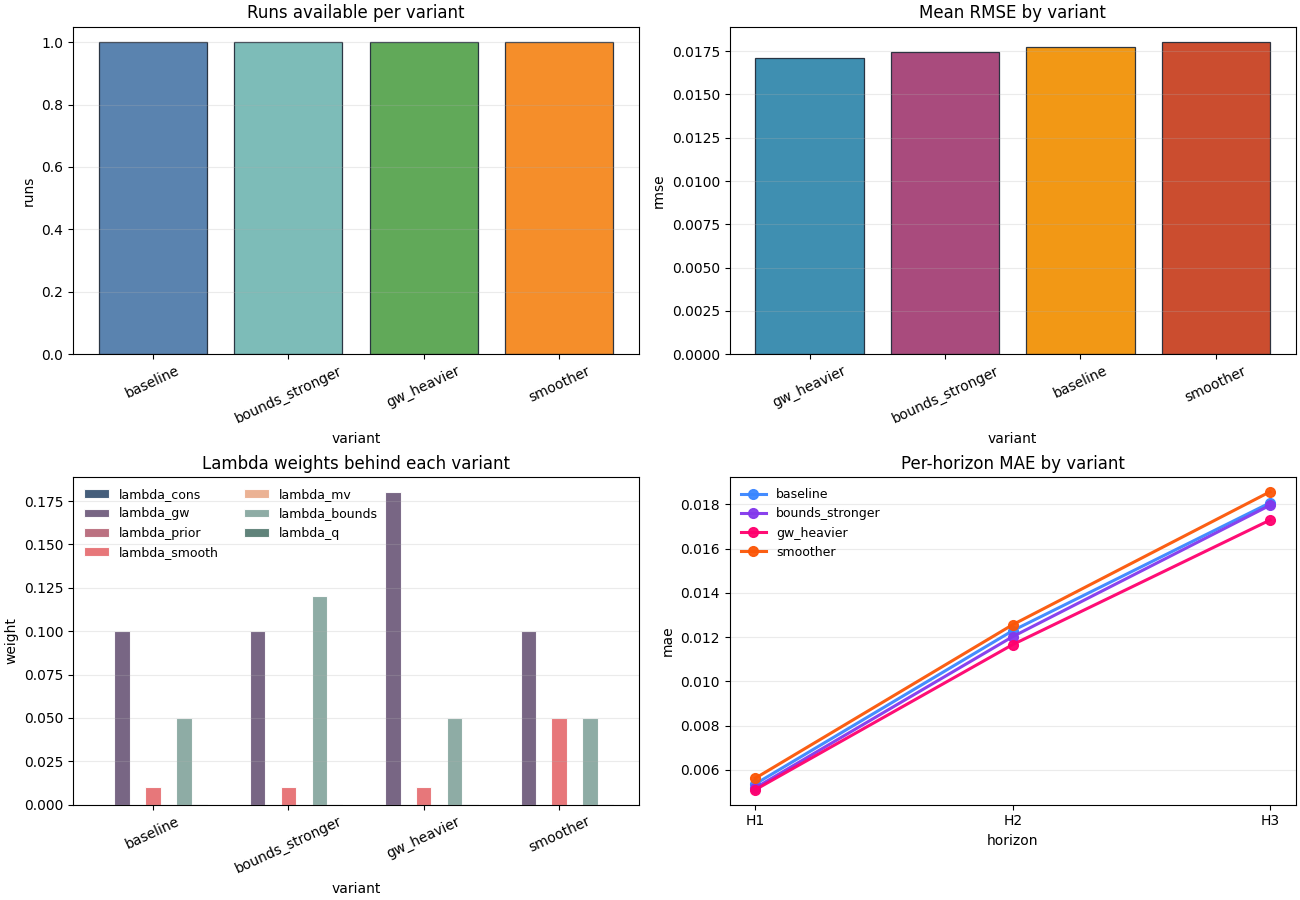
Plot the main comparison views#
A compact ablation review is usually easier when we look at four complementary views:
how many runs belong to each variant,
which variants rank best on RMSE,
how the lambda weights differ,
how MAE behaves across horizons.
Notice that each plot answers a different decision question. That is much better than drawing many redundant score charts.
fig, axes = plt.subplots(
    2,
    2,
    figsize=(13.0, 9.0),
    constrained_layout=True,
)

axes[1, 0].set_prop_cycle(color=ABLATION_PALETTE["lambdas"])
axes[1, 1].set_prop_cycle(color=ABLATION_PALETTE["horizon_lines"])

plot_ablation_run_counts(
    records,
    ax=axes[0, 0],
    title="Runs available per variant",
    color=ABLATION_PALETTE["counts"],
    edgecolor="#1F2937",
    linewidth=0.9,
    alpha=0.92,
)
plot_ablation_metric_by_variant(
    records,
    metric="rmse",
    ax=axes[0, 1],
    title="Mean RMSE by variant",
    color=ABLATION_PALETTE["rmse"],
    edgecolor="#1F2937",
    linewidth=0.9,
    alpha=0.92,
)
plot_ablation_lambda_weights(
    records,
    ax=axes[1, 0],
    title="Lambda weights behind each variant",
    edgecolor="white",
    linewidth=0.8,
    alpha=0.92,
    legend_kws={"ncol": 2, "frameon": False, "fontsize": 9},
)
plot_ablation_per_horizon_metric(
    records,
    metric="mae",
    ax=axes[1, 1],
    title="Per-horizon MAE by variant",
    linewidth=2.2,
    markersize=7,
    marker="o",
    alpha=0.95,
    legend_kws={"frameon": False, "fontsize": 9},
)
<Axes: title={'center': 'Per-horizon MAE by variant'}, xlabel='horizon', ylabel='mae'>
How to read these plots#
Here is a practical interpretation order:
- Run count plot
Check whether comparison is balanced. If one variant has many more runs or seeds, its mean score may be more stable than the others.
- RMSE plot
This is the quick performance ranking. It is often the first chart a reader notices, but it should never be read in isolation.
- Lambda plot
This explains what actually changed. Without this chart, a good score might look mysterious or misleading.
- Per-horizon MAE plot
This shows where the gain happens. A variant that only improves H1 but worsens H3 may not be the best operational choice.
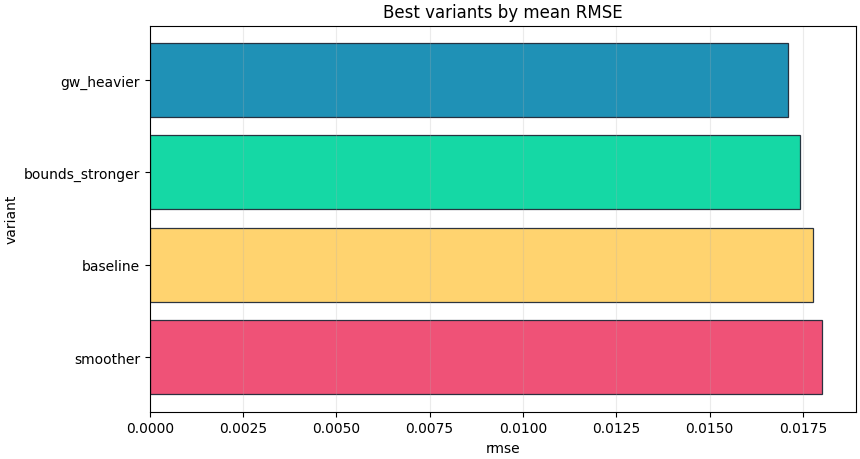
Plot the best-ranked variants explicitly#
The top-variants plot is useful when the file becomes longer and you want a quick shortlist. In a real workflow, this is often the chart that helps decide which configurations deserve a rerun, deeper diagnosis, or reporting.
fig, ax = plt.subplots(
    figsize=(8.6, 4.6),
    constrained_layout=True,
)
plot_ablation_top_variants(
    records,
    metric="rmse",
    top_n=4,
    ax=ax,
    title="Best variants by mean RMSE",
    color=ABLATION_PALETTE["top"],
    edgecolor="#1F2937",
    linewidth=0.9,
    alpha=0.94,
)
<Axes: title={'center': 'Best variants by mean RMSE'}, xlabel='rmse', ylabel='variant'>
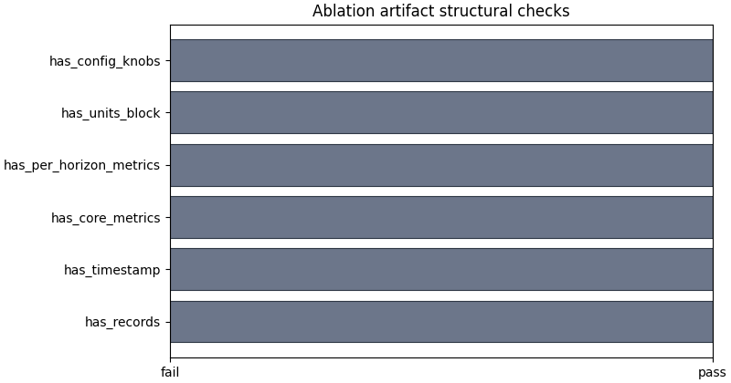
Plot the structural checks separately#
The boolean summary is a small but useful guardrail. It tells us whether the file carries the minimum information needed for a real comparison: records, metrics, horizon metrics, units, and config knobs.
fig, ax = plt.subplots(
    figsize=(8.0, 4.2),
    constrained_layout=True,
)
plot_ablation_boolean_summary(
    records,
    ax=ax,
    title="Ablation artifact structural checks",
    color=ABLATION_PALETTE["checks"],
    edgecolor="#1F2937",
    linewidth=0.8,
    alpha=0.9,
)
<Axes: title={'center': 'Ablation artifact structural checks'}>
Save the full inspection bundle#
The all-in-one inspector is useful when you want to keep the semantic summary, tidy frames, and saved figures together. This is a convenient pattern for reports, gallery generation, or later CLI helpers that may inspect a whole experiment folder.
bundle_dir = out_dir / "inspection_bundle"
bundle = inspect_ablation_record(
    records,
    output_dir=bundle_dir,
    stem="lesson_ablation",
    save_figures=True,
)

print("\nSaved inspection figures")
for name, path in bundle["figure_paths"].items():
    print(f" - {name}: {path}")
Saved inspection figures
 - lesson_ablation_run_counts.png: /tmp/gp_ablation_nxwhtrru/inspection_bundle/lesson_ablation_run_counts.png
 - lesson_ablation_rmse.png: /tmp/gp_ablation_nxwhtrru/inspection_bundle/lesson_ablation_rmse.png
 - lesson_ablation_r2.png: /tmp/gp_ablation_nxwhtrru/inspection_bundle/lesson_ablation_r2.png
 - lesson_ablation_lambda_weights.png: /tmp/gp_ablation_nxwhtrru/inspection_bundle/lesson_ablation_lambda_weights.png
 - lesson_ablation_per_h_mae.png: /tmp/gp_ablation_nxwhtrru/inspection_bundle/lesson_ablation_per_h_mae.png
 - lesson_ablation_checks.png: /tmp/gp_ablation_nxwhtrru/inspection_bundle/lesson_ablation_checks.png
A practical decision rule#
A simple reading rule for ablation records can be:
choose variants with strong scalar fit metrics,
reject variants whose horizon-wise behavior degrades badly,
reject variants whose epsilon diagnostics become suspicious,
and always confirm the configuration knobs that changed.
In this demo, the most plausible candidate is the one that combines a good RMSE ranking with stable horizon behavior and no obvious structural warning.
best = summary.get("best_by_rmse") or {}
best_variant = best.get("variant")

print("\nDecision note")
if best_variant:
    print(
        "A good next candidate for deeper review is: "
        f"{best_variant!r}. But the final choice should still "
        "consider horizon-wise behavior and epsilon diagnostics, "
        "not only the scalar RMSE ranking."
    )
else:
    print(
        "No clear best variant could be identified from the "
        "available ablation records."
    )
Decision note
A good next candidate for deeper review is: 'gw_heavier'. But the final choice should still consider horizon-wise behavior and epsilon diagnostics, not only the scalar RMSE ranking.
Total running time of the script: (0 minutes 1.599 seconds)