
Note
Go to the end to download the full example code.
Interval calibration with calibrate_quantile_forecasts#
This lesson introduces one of the most important uncertainty utilities
in GeoPrior:
geoprior.utils.calibrate.calibrate_quantile_forecasts().
Why this page matters#
A forecast can be visually impressive and still be poorly calibrated.
For quantile forecasts, a central question is:
Do the predictive intervals contain the truth as often as they claim?
For example, if we use the q10-q90 interval as an 80% interval, then we expect the observed value to fall inside that band about 80% of the time. If it falls inside much less often, the intervals are too narrow and the forecast is overconfident.
That is the problem this utility addresses.
The calibration workflow in GeoPrior is built around three closely connected helpers:
fit_interval_factors_df: fit a widening factor per horizon step so the interval coverage approaches a target;apply_interval_factors_df: widen or shrink the quantile columns around the median;calibrate_quantile_forecasts: the high-level wrapper that fits or accepts factors, applies them to evaluation and future forecasts, and returns summary statistics.
The lower-level factor fitter groups by forecast step, estimates a factor per horizon, and targets a requested coverage level. The application helper then rescales lower and upper quantiles around the median and can enforce monotonic quantile ordering. The wrapper adds automatic skip logic and before/after summaries.
What this lesson teaches#
We will:
build a synthetic evaluation and future forecast table,
deliberately make the raw intervals too narrow,
measure coverage and sharpness before calibration,
fit horizon-wise interval factors,
apply them manually,
repeat the same workflow with the high-level wrapper,
build explanatory plots showing why the calibration is useful.
This lesson is intentionally synthetic so it remains fully executable during the documentation build.
Imports#
We use the real uncertainty helpers from GeoPrior.
from __future__ import annotations

import numpy as np
import pandas as pd
import matplotlib.pyplot as plt

from geoprior.utils.calibrate import (
    apply_interval_factors_df,
    calibrate_quantile_forecasts,
    fit_interval_factors_df,
)
Step 1 - Build synthetic forecast tables#
We create:
df_eval: evaluation rows with actual values available;df_future: future rows with predictions only.
Each row represents one spatial sample at one forecast step.
We deliberately make the q10-q90 intervals too narrow so that the initial empirical coverage is below the nominal 80% target.
rng = np.random.default_rng(7)

nx = 9
ny = 6
steps = [1, 2, 3]
future_years = {1: 2024, 2: 2025, 3: 2026}

xv = np.linspace(0.0, 12_000.0, nx)
yv = np.linspace(0.0, 8_000.0, ny)
X, Y = np.meshgrid(xv, yv)

x_flat = X.ravel()
y_flat = Y.ravel()
n_sites = x_flat.size

xn = (x_flat - x_flat.min()) / (x_flat.max() - x_flat.min())
yn = (y_flat - y_flat.min()) / (y_flat.max() - y_flat.min())

hotspot = np.exp(
    -(
        ((xn - 0.72) ** 2) / 0.020
        + ((yn - 0.34) ** 2) / 0.030
    )
)
ridge = 0.50 * np.exp(
    -(
        ((xn - 0.26) ** 2) / 0.030
        + ((yn - 0.74) ** 2) / 0.050
    )
)
gradient = 0.44 * xn + 0.20 * (1.0 - yn)

eval_rows: list[dict[str, float | int]] = []
future_rows: list[dict[str, float | int]] = []

for step in steps:
    scale = {1: 1.00, 2: 1.18, 3: 1.40}[step]

    q50 = (
        2.2
        + 1.4 * gradient
        + 2.0 * hotspot
        + 0.9 * ridge
    ) * scale

    # Deliberately too narrow intervals
    width_raw = (
        0.12
        + 0.04 * xn
        + 0.02 * hotspot
        + 0.02 * step
    )

    q10 = q50 - width_raw
    q90 = q50 + width_raw

    # Truth is noisier than the interval expects -> undercoverage
    actual = q50 + rng.normal(0.0, 0.22 + 0.05 * step, size=n_sites)

    for i in range(n_sites):
        eval_rows.append(
            {
                "sample_idx": i,
                "forecast_step": step,
                "coord_t": future_years[step],
                "coord_x": float(x_flat[i]),
                "coord_y": float(y_flat[i]),
                "subsidence_q10": float(q10[i]),
                "subsidence_q50": float(q50[i]),
                "subsidence_q90": float(q90[i]),
                "subsidence_actual": float(actual[i]),
            }
        )

    # Future forecast uses the same raw uncertainty pattern but no actuals
    q50_future = q50 * 1.06
    q10_future = q50_future - width_raw
    q90_future = q50_future + width_raw

    for i in range(n_sites):
        future_rows.append(
            {
                "sample_idx": i,
                "forecast_step": step,
                "coord_t": future_years[step] + 1,
                "coord_x": float(x_flat[i]),
                "coord_y": float(y_flat[i]),
                "subsidence_q10": float(q10_future[i]),
                "subsidence_q50": float(q50_future[i]),
                "subsidence_q90": float(q90_future[i]),
            }
        )

df_eval = pd.DataFrame(eval_rows)
df_future = pd.DataFrame(future_rows)

print("df_eval shape:", df_eval.shape)
print("df_future shape:", df_future.shape)
print("")
print(df_eval.head(8).to_string(index=False))
df_eval shape: (162, 9)
df_future shape: (162, 8)

 sample_idx  forecast_step  coord_t    coord_x  coord_y  subsidence_q10  subsidence_q50  subsidence_q90  subsidence_actual
          0              1     2024     0.0000   0.0000          2.3400          2.4800          2.6200             2.4803
          1              1     2024  1500.0000   0.0000          2.4120          2.5570          2.7020             2.6377
          2              1     2024  3000.0000   0.0000          2.4840          2.6340          2.7840             2.5600
          3              1     2024  4500.0000   0.0000          2.5561          2.7111          2.8661             2.4707
          4              1     2024  6000.0000   0.0000          2.6317          2.7918          2.9518             2.6690
          5              1     2024  7500.0000   0.0000          2.7267          2.8920          3.0573             2.6243
          6              1     2024  9000.0000   0.0000          2.8121          2.9826          3.1530             2.9988
          7              1     2024 10500.0000   0.0000          2.8566          3.0318          3.2069             3.3936
Step 2 - Compute empirical coverage and sharpness before calibration#
Calibration is about matching observed coverage to nominal coverage.
For the q10-q90 interval we treat the nominal target as 80%.
We compute:
empirical coverage: fraction of actual values inside [q10, q90],
sharpness: average interval width q90 - q10.
These two numbers should always be read together.
Wider intervals often improve coverage.
Narrower intervals often reduce coverage.
Good uncertainty quantification balances both.
def coverage_and_width(
    df: pd.DataFrame,
    *,
    lo_col: str = "subsidence_q10",
    hi_col: str = "subsidence_q90",
    actual_col: str = "subsidence_actual",
) -> tuple[float, float]:
    yt = df[actual_col].to_numpy(float)
    lo = df[lo_col].to_numpy(float)
    hi = df[hi_col].to_numpy(float)
    covered = (yt >= lo) & (yt <= hi)
    coverage = float(np.mean(covered))
    width = float(np.mean(hi - lo))
    return coverage, width


before_rows = []
for step, g in df_eval.groupby("forecast_step", sort=True):
    cov, wid = coverage_and_width(g)
    before_rows.append(
        {
            "forecast_step": int(step),
            "coverage_before": cov,
            "sharpness_before": wid,
        }
    )

df_before = pd.DataFrame(before_rows)

print("")
print("Before calibration")
print(df_before.to_string(index=False))
Before calibration
 forecast_step  coverage_before  sharpness_before
             1           0.4815            0.3223
             2           0.4815            0.3623
             3           0.4444            0.4023
Interpretation#
In this synthetic example, the empirical coverage should be below the intended 0.80 target for at least some horizon steps.
That is the uncertainty problem we want to fix: the forecast intervals are too sharp relative to the observed residual spread.
Step 3 - Fit interval factors with the low-level helper#
fit_interval_factors_df estimates one factor per horizon step.
Conceptually, each factor rescales the interval around the median:
lower quantiles move farther below q50,
upper quantiles move farther above q50.
The function groups by forecast_step and uses a bisection search
so the empirical coverage approaches the requested target.
factors = fit_interval_factors_df(
    df_eval,
    target_name="subsidence",
    step_col="forecast_step",
    interval=(0.1, 0.9),
    target_coverage=0.8,
    median_q=0.5,
    verbose=0,
)

print("")
print("Fitted factors by horizon")
print(factors)
Fitted factors by horizon
{1: 2.037485122680664, 2: 2.0255374908447266, 3: 1.9699583053588867}
How to read the factors#
The factor is interpreted around the median:
factor > 1: widen the interval,
factor = 1: leave the interval unchanged,
factor < 1: shrink the interval.
In undercovered forecasts, we usually expect factors larger than 1.
Step 4 - Apply interval factors manually#
apply_interval_factors_df is the second low-level helper.
It rescales all quantiles around the median and can enforce monotonic
ordering of the quantiles using strategies such as cummax or
sort. It also stores the applied factor and marks the forecast as
calibrated.
df_eval_manual = apply_interval_factors_df(
    df_eval,
    factors,
    target_name="subsidence",
    step_col="forecast_step",
    keep_original=True,
    factor_col="calibration_factor",
    calibrated_col="is_calibrated",
    enforce_monotonic="cummax",
    verbose=0,
)

df_future_manual = apply_interval_factors_df(
    df_future,
    factors,
    target_name="subsidence",
    step_col="forecast_step",
    keep_original=True,
    factor_col="calibration_factor",
    calibrated_col="is_calibrated",
    enforce_monotonic="cummax",
    verbose=0,
)

after_rows = []
for step, g in df_eval_manual.groupby("forecast_step", sort=True):
    cov, wid = coverage_and_width(g)
    after_rows.append(
        {
            "forecast_step": int(step),
            "coverage_after": cov,
            "sharpness_after": wid,
        }
    )

df_after = pd.DataFrame(after_rows)

df_compare = df_before.merge(df_after, on="forecast_step")
print("")
print("Before/after manual calibration")
print(df_compare.to_string(index=False))
Before/after manual calibration
 forecast_step  coverage_before  sharpness_before  coverage_after  sharpness_after
             1           0.4815            0.3223          0.8148           0.6566
             2           0.4815            0.3623          0.8148           0.7338
             3           0.4444            0.4023          0.8148           0.7925
What changed#
After calibration:
coverage should move closer to the target 0.80,
sharpness will usually increase because the interval has widened.
This is the central trade-off in interval calibration.
Step 5 - Run the high-level wrapper#
calibrate_quantile_forecasts packages the full workflow:
optional auto-skip if already calibrated,
use user-supplied factors or fit from
df_eval,apply to both
df_evalanddf_future,return a stats dictionary with before/after summaries.
This is the function that should be taught first in the uncertainty gallery because it naturally explains the two helper functions as part of one coherent pipeline.
df_eval_cal, df_future_cal, stats = calibrate_quantile_forecasts(
    df_eval=df_eval,
    df_future=df_future,
    target_name="subsidence",
    step_col="forecast_step",
    interval=(0.1, 0.9),
    target_coverage=0.8,
    median_q=0.5,
    use="auto",
    tol=0.02,
    keep_original=True,
    enforce_monotonic="cummax",
    verbose=0,
)

print("")
print("Calibration stats")
print(stats)
Calibration stats
{'target': 0.8, 'interval': [0.1, 0.9], 'f_max': 5.0, 'tol': 0.02, 'overall_key': '__overall__', 'factors_source': 'fit', 'factors': {'1': 2.037485122680664, '2': 2.0255374908447266, '3': 1.9699583053588867}, 'eval_before': {'coverage': 0.4691358024691358, 'sharpness': 0.3622788281364486, 'per_horizon': {'1': {'coverage': 0.48148148148148145, 'sharpness': 0.3222788281364486}, '2': {'coverage': 0.48148148148148145, 'sharpness': 0.36227882813644857}, '3': {'coverage': 0.4444444444444444, 'sharpness': 0.4022788281364487}}}, 'eval_after': {'coverage': 0.8148148148148148, 'sharpness': 0.7276400615900265, 'per_horizon': {'1': {'coverage': 0.8148148148148148, 'sharpness': 0.6566383176829725}, '2': {'coverage': 0.8148148148148148, 'sharpness': 0.7338093485296703}, '3': {'coverage': 0.8148148148148148, 'sharpness': 0.792472518557437}}}}
Why this wrapper is useful#
The wrapper adds several practical behaviors that matter in real workflows:
it can skip calibration if the evaluation intervals already look calibrated;
it can use fixed user factors instead of refitting;
it can save calibrated eval/future tables and JSON stats;
it summarizes coverage and sharpness before and after calibration.
Step 6 - Build compact explanatory plots#
The calibration helpers themselves return DataFrames and dictionaries, not figures. But lesson pages become much easier to understand when we turn the returned information into small diagnostic plots.
We build two plots:
coverage before vs after by horizon,
sharpness before vs after by horizon.
This makes the calibration trade-off visible immediately.
stats_before = stats["eval_before"]["per_horizon"]
stats_after = stats["eval_after"]["per_horizon"]

plot_rows = []
for h in sorted(stats_before, key=lambda x: int(x)):
    plot_rows.append(
        {
            "forecast_step": int(h),
            "coverage_before": stats_before[h]["coverage"],
            "coverage_after": stats_after[h]["coverage"],
            "sharpness_before": stats_before[h]["sharpness"],
            "sharpness_after": stats_after[h]["sharpness"],
        }
    )

df_plot = pd.DataFrame(plot_rows)

fig, axes = plt.subplots(1, 2, figsize=(11, 4.2))

axes[0].plot(
    df_plot["forecast_step"],
    df_plot["coverage_before"],
    marker="o",
    label="Before",
)
axes[0].plot(
    df_plot["forecast_step"],
    df_plot["coverage_after"],
    marker="s",
    label="After",
)
axes[0].axhline(0.80, linestyle="--", linewidth=1.5, label="Target 0.80")
axes[0].set_xlabel("Forecast step")
axes[0].set_ylabel("Empirical coverage")
axes[0].set_title("Coverage moves toward the target")
axes[0].grid(True, linestyle=":", alpha=0.6)
axes[0].legend()

axes[1].plot(
    df_plot["forecast_step"],
    df_plot["sharpness_before"],
    marker="o",
    label="Before",
)
axes[1].plot(
    df_plot["forecast_step"],
    df_plot["sharpness_after"],
    marker="s",
    label="After",
)
axes[1].set_xlabel("Forecast step")
axes[1].set_ylabel("Mean interval width")
axes[1].set_title("Sharper vs wider intervals")
axes[1].grid(True, linestyle=":", alpha=0.6)
axes[1].legend()

plt.tight_layout()
plt.show()
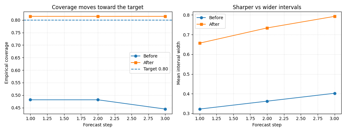
How to read these plots#
Left panel#
The goal is not necessarily to hit the target exactly at every step, but to move empirical coverage toward the desired level.
Right panel#
Better coverage usually comes at the price of wider intervals.
That is why uncertainty pages should always talk about both:
coverage: are we honest enough?
sharpness: are we still informative?
Calibration is useful when it improves honesty without exploding the interval width unnecessarily.
Step 7 - Inspect the calibrated tables directly#
The resulting forecast tables now carry explicit calibration metadata.
print("")
print("Calibrated evaluation columns")
print(df_eval_cal.columns.tolist())

print("")
print("Calibrated future head")
print(df_future_cal.head(8).to_string(index=False))
Calibrated evaluation columns
['sample_idx', 'forecast_step', 'coord_t', 'coord_x', 'coord_y', 'subsidence_q10', 'subsidence_q50', 'subsidence_q90', 'subsidence_actual', 'subsidence_q10_raw', 'subsidence_q50_raw', 'subsidence_q90_raw', 'calibration_factor', 'is_calibrated']

Calibrated future head
 sample_idx  forecast_step  coord_t    coord_x  coord_y  subsidence_q10  subsidence_q50  subsidence_q90  subsidence_q10_raw  subsidence_q50_raw  subsidence_q90_raw  calibration_factor  is_calibrated
          0              1     2025     0.0000   0.0000          2.3436          2.6288          2.9140              2.4888              2.6288              2.7688              2.0375           True
          1              1     2025  1500.0000   0.0000          2.4150          2.7104          3.0059              2.5654              2.7104              2.8554              2.0375           True
          2              1     2025  3000.0000   0.0000          2.4864          2.7920          3.0977              2.6420              2.7920              2.9420              2.0375           True
          3              1     2025  4500.0000   0.0000          2.5580          2.8738          3.1896              2.7188              2.8738              3.0288              2.0375           True
          4              1     2025  6000.0000   0.0000          2.6332          2.9593          3.2854              2.7992              2.9593              3.1193              2.0375           True
          5              1     2025  7500.0000   0.0000          2.7288          3.0655          3.4023              2.9003              3.0655              3.2308              2.0375           True
          6              1     2025  9000.0000   0.0000          2.8143          3.1615          3.5087              2.9911              3.1615              3.3319              2.0375           True
          7              1     2025 10500.0000   0.0000          2.8568          3.2137          3.5705              3.0385              3.2137              3.3888              2.0375           True
Notice two practical columns:
calibration_factor: the factor actually used for that horizon;is_calibrated: a flag that helps downstream logic detect that calibration was already applied.
This is also why the wrapper can auto-skip re-calibration later.
Step 8 - Why this page should come first in uncertainty#
This page teaches the foundational uncertainty idea in the most concrete possible way:
forecasts can be overconfident,
interval coverage can be measured directly,
intervals can be recalibrated per horizon,
future forecasts can inherit the same fitted factors.
That makes this the best first page in the uncertainty gallery.
Later pages can then build naturally on top of it:
reliability diagrams,
coverage-versus-sharpness trade-offs,
probability calibration,
exceedance-oriented uncertainty analysis.
Total running time of the script: (0 minutes 0.303 seconds)