
Note
Go to the end to download the full example code.
Build city boundary polygons from forecast points#
This example teaches you how to use GeoPrior’s
make-boundary utility.
Unlike the plotting scripts, this command is a spatial-support builder. It reads forecast point locations and turns them into simple boundary polygons that can later be reused by grid, exposure, or map-oriented workflows.
Why this matters#
Many later spatial products need a compact city footprint rather than a raw point cloud.
This builder converts forecast point coordinates into:
one boundary polygon per city,
written as GeoJSON or Shapefile,
using either a convex hull or a concave hull.
That makes it a natural lesson for the
tables_and_summaries gallery, even though the
artifact is spatial rather than tabular.
Imports#
We call the real production entrypoint from the project code. Then we read the generated boundary files back in and build one compact visual preview for the lesson page.
from __future__ import annotations

import json
import tempfile
from pathlib import Path

import geopandas as gpd
import matplotlib.pyplot as plt
import numpy as np
import pandas as pd
from shapely.geometry import shape

from geoprior.scripts.make_boundary import (
    make_boundary_main,
)
from geoprior.scripts import utils as script_utils
Build compact synthetic point clouds#
The production script only needs:
coord_x
coord_y
but for a realistic lesson page we also add:
city
sample_idx
coord_t
We create:
Nansha
Zhongshan
with one eval cloud and one future cloud per city.
The future cloud is slightly expanded relative to the eval cloud so the boundary reflects the union of both.
rng = np.random.default_rng(5)


def _city_points(
    *,
    city: str,
    center_x: float,
    center_y: float,
    scale_x: float,
    scale_y: float,
    drift_x: float,
    drift_y: float,
    n: int = 120,
) -> tuple[pd.DataFrame, pd.DataFrame]:
    ang = rng.uniform(0.0, 2.0 * np.pi, size=n)
    rad = np.sqrt(rng.uniform(0.0, 1.0, size=n))

    xe = center_x + scale_x * rad * np.cos(ang)
    ye = center_y + scale_y * rad * np.sin(ang)

    xf = (
        center_x
        + drift_x
        + 1.08 * scale_x * rad * np.cos(ang)
        + rng.normal(0.0, 3.0, size=n)
    )
    yf = (
        center_y
        + drift_y
        + 1.08 * scale_y * rad * np.sin(ang)
        + rng.normal(0.0, 2.5, size=n)
    )

    eval_df = pd.DataFrame(
        {
            "city": city,
            "sample_idx": np.arange(n, dtype=int),
            "coord_t": 2022,
            "coord_x": xe.astype(float),
            "coord_y": ye.astype(float),
        }
    )

    future_df = pd.DataFrame(
        {
            "city": city,
            "sample_idx": np.arange(n, dtype=int),
            "coord_t": 2025,
            "coord_x": xf.astype(float),
            "coord_y": yf.astype(float),
        }
    )

    return eval_df, future_df


ns_eval_df, ns_future_df = _city_points(
    city="Nansha",
    center_x=1200.0,
    center_y=800.0,
    scale_x=115.0,
    scale_y=72.0,
    drift_x=18.0,
    drift_y=10.0,
)

zh_eval_df, zh_future_df = _city_points(
    city="Zhongshan",
    center_x=1700.0,
    center_y=1050.0,
    scale_x=155.0,
    scale_y=92.0,
    drift_x=28.0,
    drift_y=14.0,
)

print("Nansha eval preview")
print(ns_eval_df.head(6).to_string(index=False))

print("")
print("Zhongshan future preview")
print(zh_future_df.head(6).to_string(index=False))
Nansha eval preview
  city  sample_idx  coord_t   coord_x  coord_y
Nansha           0     2022 1236.1009 737.2232
Nansha           1     2022 1223.7811 760.9249
Nansha           2     2022 1098.0242 793.8330
Nansha           3     2022 1183.7973 844.3333
Nansha           4     2022 1283.5959 818.4467
Nansha           5     2022 1126.5943 841.3625

Zhongshan future preview
     city  sample_idx  coord_t   coord_x   coord_y
Zhongshan           0     2025 1783.7960  987.8269
Zhongshan           1     2025 1833.9731 1095.5350
Zhongshan           2     2025 1700.3008 1092.0056
Zhongshan           3     2025 1801.9069 1117.2066
Zhongshan           4     2025 1694.2890 1079.6684
Zhongshan           5     2025 1693.7081 1077.9448
Write the lesson inputs#
We use explicit per-city eval/future CSVs here. That keeps the lesson self-contained while still following the real command’s file-based workflow.
tmp_dir = Path(
    tempfile.mkdtemp(prefix="gp_sg_boundary_")
)

ns_eval_csv = tmp_dir / "nansha_eval.csv"
ns_future_csv = tmp_dir / "nansha_future.csv"
zh_eval_csv = tmp_dir / "zhongshan_eval.csv"
zh_future_csv = tmp_dir / "zhongshan_future.csv"

ns_eval_df.to_csv(ns_eval_csv, index=False)
ns_future_df.to_csv(ns_future_csv, index=False)
zh_eval_df.to_csv(zh_eval_csv, index=False)
zh_future_df.to_csv(zh_future_csv, index=False)

print("")
print("Input files")
for p in [
    ns_eval_csv,
    ns_future_csv,
    zh_eval_csv,
    zh_future_csv,
]:
    print(" -", p.name)
Input files
 - nansha_eval.csv
 - nansha_future.csv
 - zhongshan_eval.csv
 - zhongshan_future.csv
Run the real boundary builder#
We ask the production command to:
use explicit city CSVs,
build convex hull boundaries,
write GeoJSON outputs,
and honor an explicit parent folder.
New output semantics:
bare relative names go to scripts/out,
relative or absolute paths with a parent are kept as given.
Here we intentionally pass a nested folder so the example teaches the override behavior.
out_stem = (tmp_dir / "exports" / "boundary_gallery").resolve()
out_stem.parent.mkdir(parents=True, exist_ok=True)

written = make_boundary_main(
    [
        "--ns-eval",
        str(ns_eval_csv),
        "--ns-future",
        str(ns_future_csv),
        "--zh-eval",
        str(zh_eval_csv),
        "--zh-future",
        str(zh_future_csv),
        "--method",
        "convex",
        "--format",
        "geojson",
        "--out",
        str(out_stem),
    ],
    prog="make-boundary",
) or []
[OK] wrote /tmp/gp_sg_boundary_n2bxvx6g/exports/boundary_gallery_nansha.geojson
[OK] wrote /tmp/gp_sg_boundary_n2bxvx6g/exports/boundary_gallery_zhongshan.geojson
Inspect the produced artifacts#
The builder now returns concrete paths, but we still keep a small fallback resolver so the page stays robust.
print("")
print("Written files")
for p in written:
    print(" -", p)

print("")
print("Bare-name example path")
print(" -", script_utils.resolve_out_out("boundary"))
print("Explicit-folder example stem")
print(" -", out_stem)


def _slug_city(city: str) -> str:
    return str(city).strip().lower().replace(" ", "_")


def _expected_boundary_path(
    out_stem: Path,
    city: str,
) -> Path:
    stem = out_stem.with_suffix("")
    slug = _slug_city(city)
    return stem.parent / f"{stem.name}_{slug}.geojson"


def _resolve_boundary_path(
    *,
    city: str,
    written: list[Path],
    out_stem: Path,
) -> Path:
    slug = _slug_city(city)

    for p in written:
        pp = Path(p)
        if (
            pp.suffix.lower() == ".geojson"
            and slug in pp.name.lower()
            and pp.exists()
        ):
            return pp

    cand = _expected_boundary_path(out_stem, city)
    if cand.exists():
        return cand

    raise FileNotFoundError(
        f"{city}: boundary GeoJSON not found. "
        f"Tried: {cand}. Returned: {written}"
    )


ns_boundary_path = _resolve_boundary_path(
    city="Nansha",
    written=written,
    out_stem=out_stem,
)
zh_boundary_path = _resolve_boundary_path(
    city="Zhongshan",
    written=written,
    out_stem=out_stem,
)
Written files
 - /tmp/gp_sg_boundary_n2bxvx6g/exports/boundary_gallery_nansha.geojson
 - /tmp/gp_sg_boundary_n2bxvx6g/exports/boundary_gallery_zhongshan.geojson

Bare-name example path
 - /home/docs/checkouts/readthedocs.org/user_builds/geoprior-v3/checkouts/latest/scripts/out/boundary
Explicit-folder example stem
 - /tmp/gp_sg_boundary_n2bxvx6g/exports/boundary_gallery
Read the generated boundaries#
We read both GeoJSON files back in so the page can preview the actual artifact, not just the input points.
def _read_boundary_geojson(
    path: Path,
    city: str,
) -> gpd.GeoDataFrame:
    with path.open("r", encoding="utf-8") as f:
        obj = json.load(f)

    feat = obj["features"][0]
    geom = shape(feat["geometry"])
    props = feat.get("properties", {})

    return gpd.GeoDataFrame(
        [{"city": props.get("city", city)}],
        geometry=[geom],
        crs=None,
    )


print("exists ns:", ns_boundary_path.exists())
print("exists zh:", zh_boundary_path.exists())

ns_boundary = _read_boundary_geojson(
    ns_boundary_path,
    "Nansha",
)
zh_boundary = _read_boundary_geojson(
    zh_boundary_path,
    "Zhongshan",
)

print("")
print("Nansha boundary")
print(ns_boundary.to_string(index=False))

print("")
print("Zhongshan boundary")
print(zh_boundary.to_string(index=False))
exists ns: True
exists zh: True

Nansha boundary
  city                                                                                                                                                                                                                                                                                                                                geometry
Nansha POLYGON ((1236.101 737.223, 1166.631 737.69, 1126.43 750.054, 1116.021 755.084, 1094.257 777.005, 1091.853 802.97, 1100.122 834.283, 1109.91 849.29, 1162.175 876.538, 1241.838 882.785, 1264.421 877.273, 1291.068 864.838, 1328.641 838.39, 1333.706 787.092, 1327.256 779.968, 1293.192 749.823, 1264.024 743.06, 1236.101 737.223))

Zhongshan boundary
     city                                                                                                                                                                                                                                                                                                                                               geometry
Zhongshan POLYGON ((1662.934 961.204, 1612.044 984.099, 1566.895 1008.131, 1548.566 1051.11, 1552.304 1076.748, 1567.314 1093.255, 1642.782 1146.131, 1773.62 1156.395, 1797.853 1142.709, 1811.592 1133.698, 1869.098 1093.723, 1873.67 1089.071, 1880.567 1053.263, 1871.168 1019.437, 1803.828 981.729, 1795.929 979.038, 1763.86 969.746, 1662.934 961.204))
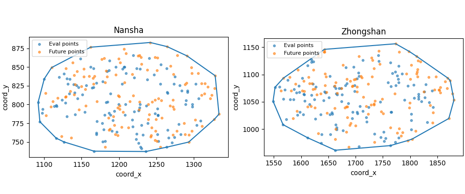
Build one compact visual preview#
This preview is not part of the production builder itself. It is a teaching aid for the gallery page.
- Left:
Nansha eval+future points with the generated boundary.
- Right:
Zhongshan eval+future points with the generated boundary.
fig, axes = plt.subplots(
    1,
    2,
    figsize=(9.6, 4.0),
    constrained_layout=True,
)

for ax, city, dfe, dff, gdf in [
    (axes[0], "Nansha", ns_eval_df, ns_future_df, ns_boundary),
    (
        axes[1],
        "Zhongshan",
        zh_eval_df,
        zh_future_df,
        zh_boundary,
    ),
]:
    ax.scatter(
        dfe["coord_x"].to_numpy(float),
        dfe["coord_y"].to_numpy(float),
        s=10,
        alpha=0.6,
        label="Eval points",
    )
    ax.scatter(
        dff["coord_x"].to_numpy(float),
        dff["coord_y"].to_numpy(float),
        s=10,
        alpha=0.6,
        label="Future points",
    )
    gdf.boundary.plot(ax=ax)
    ax.set_title(city)
    ax.set_xlabel("coord_x")
    ax.set_ylabel("coord_y")
    ax.legend(fontsize=8)
Learn how to read this builder#
This command is very literal:
collect point coordinates,
merge eval and future point sets,
wrap those points in a polygon,
write the polygon as a reusable spatial file.
It does not compute forecast statistics or hotspot scores. It only builds a footprint.
Convex vs concave hull#
The script supports two boundary styles.
convexthe smallest convex polygon that contains all points.
concavea tighter hull that can follow inward shape changes more closely, using Shapely’s
concave_hull.
The convex option is usually the safest first choice for lesson pages because it is robust and easy to interpret.
Why the union of eval and future points matters#
The script does not use only one file. It stacks:
eval coordinates,
and future coordinates.
That is useful because the final spatial footprint should reflect the full forecast- support domain, not just one split of it.
Why the lesson uses explicit CSV inputs#
In production, the command can also auto- discover per-city eval and future CSVs from a source folder, with:
--split autopreferring test files when both test and future-test artifacts are present,otherwise falling back to validation files.
For a gallery lesson, explicit CSVs are easier because they keep the example fully reproducible in one page.
Output path rules#
The builder always writes one file per city and appends the city name to the requested output stem.
So an output stem like:
boundary_gallery
becomes:
boundary_gallery_nansha.geojsonboundary_gallery_zhongshan.geojson
in multi-city mode.
Path resolution now follows two simple rules:
--out boundarywrites underscripts/out--out results/boundarykeeps theresultsfolder
This lesson uses the second form on purpose.
Why this page belongs in tables_and_summaries#
This builder produces a support artifact that later steps can reuse:
a district grid can be clipped to the boundary,
map plots can use the boundary as a visual frame,
and sample-to-zone assignment can be checked against the same footprint.
So this page is best understood as a workflow lesson, not a figure lesson.
Command-line version#
The same lesson can be reproduced from the CLI.
Legacy dispatcher, default output folder:
python -m scripts make-boundary \
  --ns-eval results/nansha_eval.csv \
  --ns-future results/nansha_future.csv \
  --zh-eval results/zhongshan_eval.csv \
  --zh-future results/zhongshan_future.csv \
  --method convex \
  --format geojson \
  --out boundary
Modern CLI, explicit output folder:
geoprior build boundary \
  --ns-eval results/nansha_eval.csv \
  --ns-future results/nansha_future.csv \
  --zh-eval results/zhongshan_eval.csv \
  --zh-future results/zhongshan_future.csv \
  --method convex \
  --format geojson \
  --out results/boundary_gallery
Source-folder discovery:
geoprior build boundary \
  --ns-src results/nansha_run \
  --zh-src results/zhongshan_run \
  --split auto \
  --method concave \
  --alpha 0.2 \
  --format both \
  --out results/boundary
The gallery page teaches the builder. The command line reproduces it in a workflow.
Total running time of the script: (0 minutes 0.543 seconds)