Plot training history with robust grouping and scale handling

This example teaches you how to use GeoPrior’s plot_history_in helper.

Unlike the plot scripts in figure_generation/, this function is a small model-inspection utility. It is designed for training logs and history dictionaries rather than paper-ready figure builders.

Why this matters

Training histories often contain a mixture of:

• headline losses,

• task-specific losses,

• physics diagnostics,

• validation curves,

• and sometimes values that cross zero.

This helper makes those histories easier to inspect because it:

• accepts History-like or dict-like inputs,

• groups metrics automatically or from user-defined groups,

• auto-adds validation curves,

• and handles log-like scaling safely.

Imports

We call the real plotting helper from the package and feed it a compact synthetic history dictionary.

from __future__ import annotations

import tempfile
from pathlib import Path

import numpy as np

from geoprior.models import plot_history

Build a compact synthetic training history

The helper accepts either:

• a Keras History object,

• a plain dict,

• or any object exposing .history as a dict.

For the lesson page, a plain dict is the simplest choice.

We include:

• total losses,

• task losses,

• physics losses,

• epsilon diagnostics,

• validation curves.

The epsilon series intentionally includes values near zero and a small negative value so the requested log scale will safely fall back to symlog for that subplot.

epochs = np.arange(1, 13, dtype=int)

loss = np.array(
    [
        2.40,
        1.92,
        1.55,
        1.28,
        1.06,
        0.92,
        0.82,
        0.74,
        0.68,
        0.64,
        0.61,
        0.58,
    ],
    dtype=float,
)

val_loss = np.array(
    [
        2.55,
        2.05,
        1.68,
        1.42,
        1.20,
        1.06,
        0.96,
        0.90,
        0.86,
        0.83,
        0.81,
        0.80,
    ],
    dtype=float,
)

history = {
    "loss": loss.tolist(),
    "val_loss": val_loss.tolist(),
    "subs_pred_loss": (
        0.74 * loss + 0.02 * np.sin(epochs)
    ).tolist(),
    "val_subs_pred_loss": (
        0.77 * val_loss + 0.02 * np.cos(epochs)
    ).tolist(),
    "gwl_pred_loss": (
        0.46 * loss + 0.02 * np.cos(epochs / 2.0)
    ).tolist(),
    "val_gwl_pred_loss": (
        0.48 * val_loss + 0.02 * np.sin(epochs / 2.0)
    ).tolist(),
    "physics_loss": (
        np.array(
            [
                0.82,
                0.64,
                0.49,
                0.37,
                0.28,
                0.22,
                0.18,
                0.15,
                0.13,
                0.12,
                0.11,
                0.10,
            ]
        )
    ).tolist(),
    "physics_loss_scaled": (
        np.array(
            [
                0.40,
                0.33,
                0.27,
                0.21,
                0.17,
                0.14,
                0.12,
                0.11,
                0.10,
                0.095,
                0.090,
                0.086,
            ]
        )
    ).tolist(),
    "epsilon_prior": (
        np.array(
            [
                0.21,
                0.17,
                0.13,
                0.09,
                0.06,
                0.04,
                0.02,
                0.01,
                0.005,
                0.000,
                -0.003,
                0.002,
            ]
        )
    ).tolist(),
    "epsilon_cons": (
        np.array(
            [
                0.16,
                0.13,
                0.10,
                0.08,
                0.06,
                0.045,
                0.032,
                0.020,
                0.012,
                0.008,
                0.004,
                0.002,
            ]
        )
    ).tolist(),
}

print("History keys")
for k in history:
    print(" -", k)

History keys
 - loss
 - val_loss
 - subs_pred_loss
 - val_subs_pred_loss
 - gwl_pred_loss
 - val_gwl_pred_loss
 - physics_loss
 - physics_loss_scaled
 - epsilon_prior
 - epsilon_cons

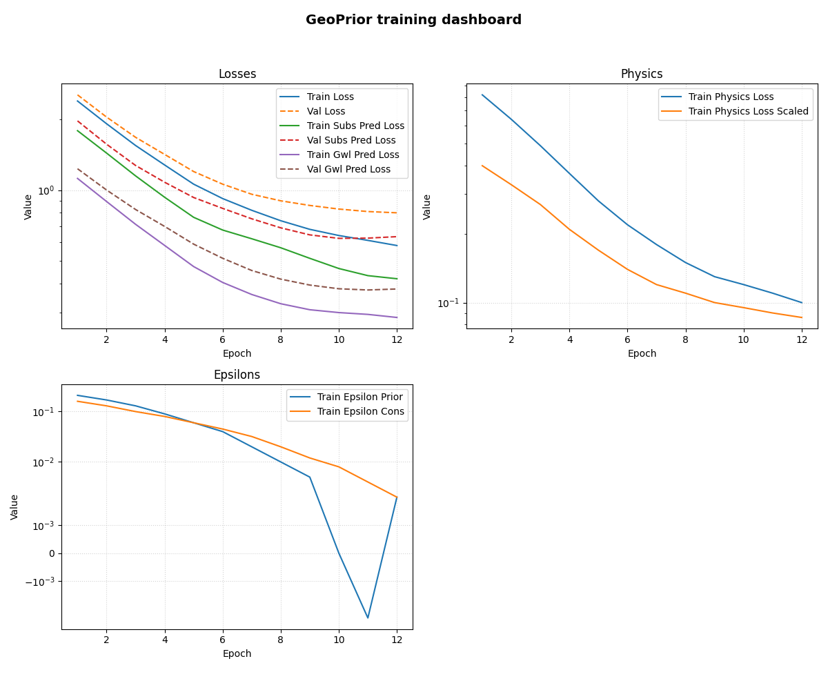
Plot a grouped inspection dashboard

Here we provide explicit groups so the figure reads like a compact training dashboard.

Two useful points to notice:

• the helper automatically adds validation curves for the non-val keys in each group;

• the epsilon panel requests log scaling, but because one series touches or crosses zero, the helper safely switches that subplot to symlog.

groups = {
    "Losses": [
        "loss",
        "subs_pred_loss",
        "gwl_pred_loss",
    ],
    "Physics": [
        "physics_loss",
        "physics_loss_scaled",
    ],
    "Epsilons": [
        "epsilon_prior",
        "epsilon_cons",
    ],
}

ysc = {
    "Losses": "log",
    "Physics": "log",
    "Epsilons": "log",
}

plot_history(
    history,
    metrics=groups,
    layout="subplots",
    title="GeoPrior training dashboard",
    max_cols=2,
    show_grid=True,
    grid_props={
        "linestyle": ":",
        "alpha": 0.55,
    },
    yscale_settings=ysc,
    linewidth=1.8,
    marker="o",
    markersize=3,
)

Let the helper auto-group the history

If metrics=None, the function creates groups automatically.

Its default rule is simple:

• keys containing loss go into a shared Losses group;

• other non-validation keys become their own titled groups.

We save that second figure to disk to demonstrate the helper’s save behavior. When the path has no extension, the function adds .png automatically.

tmp_dir = Path(
    tempfile.mkdtemp(prefix="gp_sg_plot_history_")
)
save_stem = tmp_dir / "history_autogroup"

plot_history(
    history,
    metrics=None,
    layout="subplots",
    title="Auto-grouped history view",
    max_cols=3,
    style="default",
    savefig=str(save_stem),
    linewidth=1.5,
)

saved_png = tmp_dir / "history_autogroup.png"

print("")
print("Saved file")
print(" -", saved_png)

[OK] Saved figure -> /tmp/gp_sg_plot_history_f1adi742/history_autogroup.png

Saved file
 - /tmp/gp_sg_plot_history_f1adi742/history_autogroup.png

Learn how to read the grouped dashboard

A good reading order is:

1. start with the total loss panel;

2. compare task-specific losses to see which head is harder to fit;

3. inspect the physics panel to see whether the physics objective is stabilizing;

4. inspect the epsilon panel to see whether the residual-style diagnostics are shrinking, oscillating, or crossing zero.

This is why the grouped layout is often more useful than a single all-metrics figure.

Why the safe log handling matters

Training diagnostics are often positive at the beginning and then drift toward zero, and some residual-like quantities may even cross zero.

A strict log axis would fail or hide those values. This helper instead:

• uses log when the subplot data are strictly positive;

• otherwise falls back to symlog.

That makes it much safer for physics-oriented training histories.

Why this page belongs in model_inspection

This helper is not a paper-figure script and it is not an artifact builder.

Its role is to inspect:

• optimization behavior,

• validation drift,

• and physics-diagnostic evolution

during or after training.

So it fits naturally in a model-inspection section.

A natural next lesson

After this page, the clean next lessons are:

• plot_epsilons_in.py

• plot_physics_losses_in.py

because both are thin, task-specific wrappers around plot_history_in(...).