
Note
Go to the end to download the full example code.
Spatial-block holdout as a Stage-1 diagnostic#
This lesson teaches how to use the GeoPrior holdout splitter for
train/validation/test group design, with special attention to the
"spatial_block" strategy.
We focus on:
Why this page matters#
A random split can look statistically fine and still be a weak generalization test in spatial forecasting.
If nearby points are placed into different subsets, train and test may become unrealistically similar. That is why GeoPrior supports a spatial-block strategy.
What the real utility does#
split_groups_holdout splits unique groups into train, validation,
and test subsets using either:
"random""spatial_block"
In spatial-block mode, the helper:
requires
x_colandy_col,requires
block_size > 0,bins groups into coarse (bx, by) blocks,
shuffles blocks rather than individual points,
then returns a
HoldoutSplit.
The resulting HoldoutSplit object stores the three group
tables and checks that they are disjoint.
What this lesson teaches#
We will:
build a compact spatial group table,
compare random and spatial-block splits,
check disjointness,
visualize the two splitting strategies,
explain when spatial-block holdout is preferable.
This page is synthetic so it remains fully executable during the documentation build.
Imports#
from __future__ import annotations

import numpy as np
import pandas as pd
import matplotlib.pyplot as plt

from geoprior.utils.holdout_utils import split_groups_holdout
Step 1 - Build a compact group table#
split_groups_holdout operates on a unique group table rather than
the full long temporal DataFrame.
nx = 10
ny = 7

xv = np.linspace(0.0, 12_000.0, nx)
yv = np.linspace(0.0, 8_000.0, ny)
X, Y = np.meshgrid(xv, yv)

groups = pd.DataFrame(
    {
        "group_id": np.arange(X.size),
        "coord_x": X.ravel().astype(float),
        "coord_y": Y.ravel().astype(float),
    }
)

print("Number of unique groups:", len(groups))
print("")
print(groups.head(10).to_string(index=False))
Number of unique groups: 70

 group_id      coord_x  coord_y
        0     0.000000      0.0
        1  1333.333333      0.0
        2  2666.666667      0.0
        3  4000.000000      0.0
        4  5333.333333      0.0
        5  6666.666667      0.0
        6  8000.000000      0.0
        7  9333.333333      0.0
        8 10666.666667      0.0
        9 12000.000000      0.0
Step 2 - Run the random split#
This is the simpler baseline.
split_random = split_groups_holdout(
    groups,
    seed=42,
    val_frac=0.2,
    test_frac=0.2,
    strategy="random",
)
Step 3 - Run the spatial-block split#
In spatial-block mode we must provide:
x_coly_colblock_size
split_block = split_groups_holdout(
    groups,
    seed=42,
    val_frac=0.2,
    test_frac=0.2,
    strategy="spatial_block",
    x_col="coord_x",
    y_col="coord_y",
    block_size=4000.0,
)
Step 4 - Inspect sizes and disjointness#
HoldoutSplit includes an explicit disjointness check.
split_random.check_disjoint()
split_block.check_disjoint()

summary = pd.DataFrame(
    [
        {
            "strategy": "random",
            "subset": "train",
            "n_groups": len(split_random.train_groups),
        },
        {
            "strategy": "random",
            "subset": "val",
            "n_groups": len(split_random.val_groups),
        },
        {
            "strategy": "random",
            "subset": "test",
            "n_groups": len(split_random.test_groups),
        },
        {
            "strategy": "spatial_block",
            "subset": "train",
            "n_groups": len(split_block.train_groups),
        },
        {
            "strategy": "spatial_block",
            "subset": "val",
            "n_groups": len(split_block.val_groups),
        },
        {
            "strategy": "spatial_block",
            "subset": "test",
            "n_groups": len(split_block.test_groups),
        },
    ]
)

print("")
print(summary.to_string(index=False))
     strategy subset  n_groups
       random  train        42
       random    val        14
       random   test        14
spatial_block  train        46
spatial_block    val        12
spatial_block   test        12
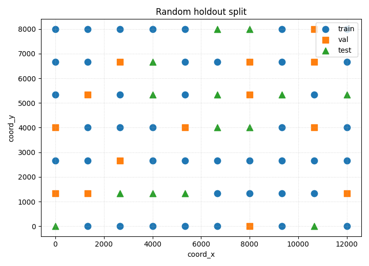
Step 5 - Plot the random split#
This shows how groups are scattered across subsets when sampling is independent.
fig, ax = plt.subplots(figsize=(7.2, 5.2))

for label, gdf, marker in [
    ("train", split_random.train_groups, "o"),
    ("val", split_random.val_groups, "s"),
    ("test", split_random.test_groups, "^"),
]:
    ax.scatter(
        gdf["coord_x"],
        gdf["coord_y"],
        marker=marker,
        s=80,
        label=label,
    )

ax.set_xlabel("coord_x")
ax.set_ylabel("coord_y")
ax.set_title("Random holdout split")
ax.grid(True, linestyle=":", alpha=0.5)
ax.legend()

plt.tight_layout()
plt.show()
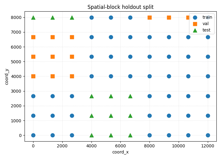
Step 6 - Plot the spatial-block split#
This view makes the block logic visible.
fig, ax = plt.subplots(figsize=(7.2, 5.2))

for label, gdf, marker in [
    ("train", split_block.train_groups, "o"),
    ("val", split_block.val_groups, "s"),
    ("test", split_block.test_groups, "^"),
]:
    ax.scatter(
        gdf["coord_x"],
        gdf["coord_y"],
        marker=marker,
        s=80,
        label=label,
    )

ax.set_xlabel("coord_x")
ax.set_ylabel("coord_y")
ax.set_title("Spatial-block holdout split")
ax.grid(True, linestyle=":", alpha=0.5)
ax.legend()

plt.tight_layout()
plt.show()
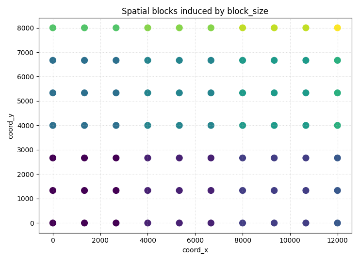
Step 7 - Visualize the coarse spatial blocks directly#
This helps explain what block_size is doing under the hood.
block_size = 4000.0

groups_with_blocks = groups.copy()
groups_with_blocks["bx"] = np.floor(
    groups_with_blocks["coord_x"] / block_size
).astype(int)
groups_with_blocks["by"] = np.floor(
    groups_with_blocks["coord_y"] / block_size
).astype(int)
groups_with_blocks["block_label"] = (
    groups_with_blocks["bx"].astype(str)
    + ","
    + groups_with_blocks["by"].astype(str)
)

block_codes = pd.factorize(groups_with_blocks["block_label"])[0]

fig, ax = plt.subplots(figsize=(7.4, 5.4))

sc = ax.scatter(
    groups_with_blocks["coord_x"],
    groups_with_blocks["coord_y"],
    c=block_codes,
    s=85,
)
ax.set_xlabel("coord_x")
ax.set_ylabel("coord_y")
ax.set_title("Spatial blocks induced by block_size")
ax.grid(True, linestyle=":", alpha=0.5)

plt.tight_layout()
plt.show()
How to read the split plots#
Random split#
Random splitting is simple and often statistically efficient, but it does not respect spatial neighborhood structure.
Spatial-block split#
Spatial-block splitting is harsher but often more realistic for geospatial generalization. Nearby points are grouped into the same holdout block, which reduces spatial leakage.
Block map#
The block visualization shows the coarse bins used before the actual
train/val/test assignment. Larger block_size makes larger spatial
neighborhoods move together.
Step 8 - Practical guidance#
Use random split when:
spatial leakage is not a major concern,
or when you need a quick baseline.
Use spatial-block split when:
the task is genuinely spatial,
nearby samples are strongly correlated,
and you want a more realistic out-of-area validation test.
This is why spatial-block holdout belongs in the diagnostics section: it defines how demanding the downstream evaluation really is.
Final takeaway#
HoldoutSplit and split_groups_holdout are not just utilities.
They define the credibility of the Stage-1 split design.
In GeoPrior, the spatial-block strategy is the diagnostic tool to use when spatial leakage would make a random split too optimistic.
Total running time of the script: (0 minutes 0.475 seconds)