
Note
Go to the end to download the full example code.
Compute hotspot summary tables from forecast CSVs#
This example teaches you how to use GeoPrior’s
compute-hotspots utility.
Unlike the figure-generation scripts, this command is an artifact builder. It reads evaluation and future forecast CSVs, compares future annual subsidence against a baseline year, and writes one compact hotspot summary table per city and year.
Why this matters#
Forecast maps can look dramatic, but downstream reporting usually needs a much more compact artifact.
This builder converts forecast CSVs into a tidy hotspot table with:
the number of hotspots,
hotspot subsidence ranges,
hotspot anomaly ranges relative to the baseline year,
the baseline mean,
and the percentile threshold used to define hotspots.
That makes it a strong lesson page for the
tables_and_summaries gallery.
Imports#
We call the real production builder, then read its outputs back in and build one compact teaching preview.
from __future__ import annotations

import tempfile
from pathlib import Path

import matplotlib.pyplot as plt
import numpy as np
import pandas as pd

import geoprior.scripts.compute_hotspots as hotspots_mod
Compatibility shim#
The current script forwards prog=... into parse_args(),
but the helper does not yet accept that keyword.
For the lesson page, we patch the helper locally so the example stays runnable. Once the script itself is patched, this shim can be removed.
_orig_parse_args = hotspots_mod.parse_args


def _parse_args_compat(
    argv: list[str] | None = None,
    *,
    prog: str | None = None,
):
    return hotspots_mod.build_parser(prog=prog).parse_args(argv)


hotspots_mod.parse_args = _parse_args_compat  # type: ignore[assignment]
Build compact synthetic cumulative forecast archives#
The production builder can work from:
explicit per-city eval and future CSVs,
or auto-discovered city source folders.
For a self-contained lesson page, we use explicit CSVs.
We generate:
Nansha
Zhongshan
with:
eval years 2021 and 2022,
future years 2023, 2024, and 2025,
cumulative subsidence columns,
and a stronger hotspot trend in Zhongshan.
This is useful because the production script’s default mode for this builder is often:
baseline year = 2022
subsidence kind = cumulative
hotspot quantile = q50
hotspot threshold = 90th percentile of anomaly magnitude
rng = np.random.default_rng(7)

eval_years = [2021, 2022]
future_years = [2023, 2024, 2025]
n_samples = 120


def _city_frames(
    *,
    city: str,
    level_shift: float,
    hotspot_boost: float,
) -> tuple[pd.DataFrame, pd.DataFrame]:
    rows_eval: list[dict[str, object]] = []
    rows_future: list[dict[str, object]] = []

    hotspot_ids = set(range(16))

    for sample_idx in range(n_samples):
        spatial = 4.5 * np.sin(sample_idx / 11.0)
        local = rng.normal(0.0, 1.4)

        annual_2021 = 24.0 + level_shift + 0.7 * spatial + local
        annual_2022 = 31.0 + level_shift + 0.9 * spatial + local

        is_hot = sample_idx in hotspot_ids
        hot_term = hotspot_boost if is_hot else 0.0

        annual_2023 = (
            annual_2022
            + 3.2
            + 0.6 * hot_term
            + rng.normal(0.0, 1.2)
        )
        annual_2024 = (
            annual_2023
            + 2.6
            + 0.8 * hot_term
            + rng.normal(0.0, 1.2)
        )
        annual_2025 = (
            annual_2024
            + 1.8
            + 1.0 * hot_term
            + rng.normal(0.0, 1.2)
        )

        # Build cumulative paths.
        q50_cum_2021 = annual_2021
        q50_cum_2022 = q50_cum_2021 + annual_2022
        q50_cum_2023 = q50_cum_2022 + annual_2023
        q50_cum_2024 = q50_cum_2023 + annual_2024
        q50_cum_2025 = q50_cum_2024 + annual_2025

        # Eval actuals are slightly noisy but remain monotone.
        act_annual_2021 = max(
            1.0,
            annual_2021 + rng.normal(0.0, 0.9),
        )
        act_annual_2022 = max(
            1.0,
            annual_2022 + rng.normal(0.0, 1.0),
        )
        act_cum_2021 = act_annual_2021
        act_cum_2022 = act_cum_2021 + act_annual_2022

        def _q_band(center: float, width: float) -> tuple[float, float]:
            return max(0.0, center - width), center + width

        # Eval rows.
        for year, q50, actual, width in [
            (2021, q50_cum_2021, act_cum_2021, 6.5),
            (2022, q50_cum_2022, act_cum_2022, 7.5),
        ]:
            q10, q90 = _q_band(q50, width)
            rows_eval.append(
                {
                    "city": city,
                    "sample_idx": sample_idx,
                    "coord_t": year,
                    "subsidence_actual": float(actual),
                    "subsidence_q10": float(q10),
                    "subsidence_q50": float(q50),
                    "subsidence_q90": float(q90),
                    "subsidence_unit": "mm",
                }
            )

        # Future rows.
        for year, q50, width in [
            (2023, q50_cum_2023, 9.0),
            (2024, q50_cum_2024, 10.5),
            (2025, q50_cum_2025, 12.0),
        ]:
            q10, q90 = _q_band(q50, width)
            rows_future.append(
                {
                    "city": city,
                    "sample_idx": sample_idx,
                    "coord_t": year,
                    "subsidence_q10": float(q10),
                    "subsidence_q50": float(q50),
                    "subsidence_q90": float(q90),
                    "subsidence_unit": "mm",
                }
            )

    return pd.DataFrame(rows_eval), pd.DataFrame(rows_future)


ns_eval_df, ns_future_df = _city_frames(
    city="Nansha",
    level_shift=0.0,
    hotspot_boost=4.0,
)

zh_eval_df, zh_future_df = _city_frames(
    city="Zhongshan",
    level_shift=5.5,
    hotspot_boost=7.0,
)

print("Nansha eval preview")
print(ns_eval_df.head(6).to_string(index=False))

print("")
print("Nansha future preview")
print(ns_future_df.head(6).to_string(index=False))
Nansha eval preview
  city  sample_idx  coord_t  subsidence_actual  subsidence_q10  subsidence_q50  subsidence_q90 subsidence_unit
Nansha           0     2021            23.5925         17.5017         24.0017         30.5017              mm
Nansha           0     2022            53.6026         47.5034         55.0034         62.5034              mm
Nansha           1     2021            24.8110         17.8702         24.3702         30.8702              mm
Nansha           1     2022            56.6198         48.3220         55.8220         63.3220              mm
Nansha           2     2021            23.5074         18.2172         24.7172         31.2172              mm
Nansha           2     2022            54.9296         49.0971         56.5971         64.0971              mm

Nansha future preview
  city  sample_idx  coord_t  subsidence_q10  subsidence_q50  subsidence_q90 subsidence_unit
Nansha           0     2023         82.9637         91.9637        100.9637              mm
Nansha           0     2024        123.8949        134.3949        144.8949              mm
Nansha           0     2025        169.5575        181.5575        193.5575              mm
Nansha           1     2023         85.4822         94.4822        103.4822              mm
Nansha           1     2024        127.8517        138.3517        148.8517              mm
Nansha           1     2025        175.2766        187.2766        199.2766              mm
Write the lesson inputs#
The production builder consumes CSV files, so we follow the real workflow exactly.
tmp_dir = Path(
    tempfile.mkdtemp(prefix="gp_sg_hotspots_")
)

ns_eval_csv = tmp_dir / "nansha_eval.csv"
ns_future_csv = tmp_dir / "nansha_future.csv"
zh_eval_csv = tmp_dir / "zhongshan_eval.csv"
zh_future_csv = tmp_dir / "zhongshan_future.csv"

ns_eval_df.to_csv(ns_eval_csv, index=False)
ns_future_df.to_csv(ns_future_csv, index=False)
zh_eval_df.to_csv(zh_eval_csv, index=False)
zh_future_df.to_csv(zh_future_csv, index=False)

print("")
print("Input files")
for p in [
    ns_eval_csv,
    ns_future_csv,
    zh_eval_csv,
    zh_future_csv,
]:
    print(" -", p.name)
Input files
 - nansha_eval.csv
 - nansha_future.csv
 - zhongshan_eval.csv
 - zhongshan_future.csv
Run the real hotspot builder#
We ask the production command to:
use 2022 as the baseline year,
interpret the inputs as cumulative subsidence,
use actual values for the baseline when available,
summarize 2023, 2024, and 2025,
and export both CSV and LaTeX.
The result is one compact city × year table.
out_stem = tmp_dir / "hotspots_gallery"

hotspots_mod.compute_hotspots_main(
    [
        "--ns-eval",
        str(ns_eval_csv),
        "--ns-future",
        str(ns_future_csv),
        "--zh-eval",
        str(zh_eval_csv),
        "--zh-future",
        str(zh_future_csv),
        "--baseline-year",
        "2022",
        "--percentile",
        "90",
        "--subsidence-kind",
        "cumulative",
        "--baseline-source",
        "actual",
        "--quantile",
        "q50",
        "--years",
        "2023",
        "2024",
        "2025",
        "--format",
        "both",
        "--out",
        str(out_stem),
    ],
    prog="compute-hotspots",
)
Inspect the produced artifacts#
The builder writes:
one CSV summary table,
one LaTeX sidewaystable.
That is the core artifact family for this command.
written = sorted(tmp_dir.glob("hotspots_gallery*"))

print("")
print("Written files")
for p in written:
    print(" -", p.name)
Written files
 - hotspots_gallery.csv
 - hotspots_gallery.tex
Read the generated hotspot table#
This is the main output users will usually inspect first.
tab_csv = tmp_dir / "hotspots_gallery.csv"
tab_tex = tmp_dir / "hotspots_gallery.tex"

tab = pd.read_csv(tab_csv)

print("")
print("Hotspot summary table")
print(tab.to_string(index=False))

print("")
print("LaTeX preview")
for line in tab_tex.read_text(encoding="utf-8").splitlines()[:12]:
    print(line)
Hotspot summary table
     City  Year  Hotspots_n  s_hot_min  s_hot_mean  s_hot_max  d_hot_mean  d_hot_max  mean_2022   T_0p9
   Nansha  2023          12    31.9408     39.0185    44.0507      7.1779    10.3769    31.3303  6.1956
   Nansha  2024          12    42.1282     45.3584    47.5097     12.3683    14.1385    31.3303 10.4846
   Nansha  2025          12    47.1625     50.8033    53.7864     17.8132    19.7875    31.3303 15.3173
Zhongshan  2023          12    40.1022     45.1890    50.6990      8.8040    12.0300    36.9405  7.6105
Zhongshan  2024          12    50.9522     54.6610    60.0870     15.7146    18.1200    36.9405 13.4832
Zhongshan  2025          12    60.0815     63.8033    69.7340     24.6216    27.7670    36.9405 21.5802

LaTeX preview
\begin{sidewaystable}[p]
\centering
\caption{Characteristics of forecast hotspot clusters. Hotspots are defined as locations where the absolute change in annual subsidence relative to 2022 exceeds the 90th percentile threshold $T_{0.9}$ within each city and year.}
\label{tab:hotspots}
\begin{tabular}{llrccccccc}
\toprule
& & & \multicolumn{3}{c}{Hotspot subsidence $s_{\mathrm{hot}}$} & \multicolumn{2}{c}{Hotspot anomaly $|\Delta s_{\mathrm{hot}}|$ vs.\ 2022} & Mean 2022 subsidence & $T_{0.9}$ \\
City & Year & Hotspots & \multicolumn{3}{c}{(mm yr$^{-1}$)} & \multicolumn{2}{c}{(mm yr$^{-1}$)} & (mm yr$^{-1}$) & (mm yr$^{-1}$) \\
\cmidrule(lr){4-6} \cmidrule(lr){7-8}
& & $n$ & min & mean & max & mean & max & & \\
\midrule
Nansha & 2023 & 12 & 31.9 & 39.0 & 44.1 & 7.2 & 10.4 & 31.3 & 6.2 \\
Show how cumulative inputs become annual series#
This builder supports both:
rate / increment data, where annual values are already present,
cumulative data, where annual values must be reconstructed.
For cumulative inputs, the script uses:
baseline annual 2022 = cumulative_2022 - cumulative_2021
annual 2023 = future_2023 - cumulative_2022
annual 2024 = future_2024 - future_2023
annual 2025 = future_2025 - future_2024
Below is a concrete one-sample demonstration for Nansha.
demo_sid = 0

ev0 = ns_eval_df.loc[
    ns_eval_df["sample_idx"] == demo_sid
].sort_values("coord_t")
fu0 = ns_future_df.loc[
    ns_future_df["sample_idx"] == demo_sid
].sort_values("coord_t")

cum_2021 = float(
    ev0.loc[ev0["coord_t"] == 2021, "subsidence_actual"].iloc[0]
)
cum_2022 = float(
    ev0.loc[ev0["coord_t"] == 2022, "subsidence_actual"].iloc[0]
)
fut_2023 = float(
    fu0.loc[fu0["coord_t"] == 2023, "subsidence_q50"].iloc[0]
)
fut_2024 = float(
    fu0.loc[fu0["coord_t"] == 2024, "subsidence_q50"].iloc[0]
)
fut_2025 = float(
    fu0.loc[fu0["coord_t"] == 2025, "subsidence_q50"].iloc[0]
)

annual_demo = pd.DataFrame(
    {
        "year": [2022, 2023, 2024, 2025],
        "annual_value_mm": [
            cum_2022 - cum_2021,
            fut_2023 - cum_2022,
            fut_2024 - fut_2023,
            fut_2025 - fut_2024,
        ],
    }
)

print("")
print("Annual conversion demo for one sample")
print(annual_demo.to_string(index=False))
Annual conversion demo for one sample
 year  annual_value_mm
 2022          30.0101
 2023          38.3611
 2024          42.4313
 2025          47.1625
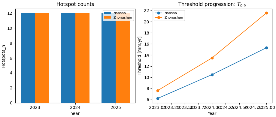
Build one compact visual preview#
This preview is not part of the production builder itself. It is a teaching aid for the gallery page.
- Left:
hotspot counts by year and city.
- Right:
the threshold T_0p9 by year and city.
fig, axes = plt.subplots(
    1,
    2,
    figsize=(9.2, 3.9),
    constrained_layout=True,
)

# Hotspot counts by year and city
ax = axes[0]
cities = ["Nansha", "Zhongshan"]
years = sorted(tab["Year"].unique())
x = np.arange(len(years))
w = 0.35

for i, city in enumerate(cities):
    vals = []
    for year in years:
        sub = tab.loc[
            (tab["City"] == city) & (tab["Year"] == year),
            "Hotspots_n",
        ]
        vals.append(float(sub.iloc[0]) if not sub.empty else np.nan)

    ax.bar(
        x + (i - 0.5) * w,
        vals,
        width=w,
        label=city,
    )

ax.set_title("Hotspot counts")
ax.set_xlabel("Year")
ax.set_ylabel("Hotspots_n")
ax.set_xticks(x)
ax.set_xticklabels([str(y) for y in years])
ax.legend(fontsize=8)

# Threshold progression
ax = axes[1]
for city in cities:
    sub = tab.loc[tab["City"] == city].sort_values("Year")
    ax.plot(
        sub["Year"].to_numpy(int),
        sub["T_0p9"].to_numpy(float),
        marker="o",
        label=city,
    )

ax.set_title(r"Threshold progression: $T_{0.9}$")
ax.set_xlabel("Year")
ax.set_ylabel("Threshold [mm/yr]")
ax.legend(fontsize=8)
<matplotlib.legend.Legend object at 0x749e56deb0e0>
Learn how to read the table#
Each row is one:
city
year
combination.
The most important columns are:
Hotspots_n: how many locations exceeded the anomaly threshold;s_hot_*: the subsidence range among hotspot points;d_hot_*: the anomaly range among hotspot points;mean_2022: the city-wide baseline annual mean for 2022;T_0p9: the percentile threshold used to define the hotspots.
So the table is not a geometry layer. It is the compact numerical summary that later reporting pages or figures can build on.
What the hotspot rule means#
For each city and year, the builder computes:
the annual baseline series for 2022,
the annual forecast series for the requested year,
the absolute anomaly:
\(\lvert future\_annual - baseline\_{2022,\mathrm{annual}} \rvert\)
Then it marks hotspots where that anomaly exceeds the chosen percentile threshold.
With the default percentile of 90, this means the most anomalous ~10 percent of valid locations become hotspots for that city-year.
Why cumulative vs rate mode matters#
This script supports two data conventions.
rateorincrementthe CSV values are already annual values.
cumulativethe CSV values are cumulative totals, so the script first converts them back to annual increments before any hotspot calculation.
That makes the builder useful for both:
already-annual forecast archives,
and future forecast exports stored in cumulative form.
Why the baseline source matters#
The baseline year can come from:
actual: use observed 2022 subsidence when available;q50: use the median forecast from the eval CSV.
In practice:
actualis better when the eval archive includes observations;q50is a useful fallback when the builder is used on a purely predictive archive.
Why this command belongs in tables_and_summaries#
This builder is a bridge between raw forecast CSVs and later presentation layers.
A useful workflow is:
generate or calibrate the forecast CSVs,
build the hotspot summary table,
inspect counts and thresholds by city and year,
only then move on to hotspot maps or narrative reporting.
That separation keeps:
forecast generation,
summary tabulation,
and visualization
clearly distinct.
Command-line version#
The same lesson can be reproduced from the CLI.
Legacy dispatcher:
python -m scripts compute-hotspots \
  --ns-eval results/nansha_eval.csv \
  --ns-future results/nansha_future.csv \
  --zh-eval results/zhongshan_eval.csv \
  --zh-future results/zhongshan_future.csv \
  --baseline-year 2022 \
  --subsidence-kind cumulative \
  --quantile q50 \
  --years 2023 2024 2025 \
  --format both \
  --out tab_hotspots
Modern CLI:
geoprior build hotspots \
  --ns-eval results/nansha_eval.csv \
  --ns-future results/nansha_future.csv \
  --zh-eval results/zhongshan_eval.csv \
  --zh-future results/zhongshan_future.csv \
  --baseline-year 2022 \
  --subsidence-kind cumulative \
  --quantile q50 \
  --years 2023 2024 2025 \
  --format both \
  --out tab_hotspots
Auto-discovery by city source folder:
geoprior build hotspots \
  --ns-src results/nansha_run \
  --zh-src results/zhongshan_run \
  --baseline-year 2022 \
  --n-years 2 \
  --format csv
The gallery page teaches the builder. The command line reproduces it in a workflow.
Total running time of the script: (0 minutes 0.311 seconds)