SM3 bounds versus ridge: learning the two main failure modes

This example teaches you how to read the GeoPrior SM3 bounds-versus-ridge summary figure.

In Supplementary Methods 3, two failure modes matter a lot:

1. clipping to bounds

2. ridge non-identifiability

These are not the same thing.

A run can hit a hard or effective bound without necessarily showing a strong ridge. And a run can show a strong ridge without obviously clipping to a bound. This figure is useful because it puts both failure modes into one compact page.

What the four panels mean

The plotting backend builds four panels:

1. bound hits counts and percentages for hits at the inferred extrema of \(K\), \(\tau\), and \(H_d\).

2. ridge distribution histogram of ridge_resid_q50 together with a threshold marking what the script calls “strong ridge”.

3. clipping versus ridge matrix a 2×2 count table showing: - not clipped / no ridge, - not clipped / strong ridge, - clipped / no ridge, - clipped / strong ridge.

4. category fractions either overall category fractions or, when lith_idx is available, stacked fractions by lithology.

Why this matters

This figure does not ask whether recovery was accurate. It asks why recovery may have failed.

That is a different question.

A model can miss the true parameters because it is pushed to the edge of the feasible region. Or it can miss them because the inverse problem is sliding along a ridge. These two situations require different scientific responses.

This gallery page builds a compact synthetic SM3-style table so the figure is fully executable during documentation builds.

Imports

We use the real plotting function and its real helper routines from the project script.

from __future__ import annotations

import json
import tempfile
from pathlib import Path

import matplotlib.image as mpimg
import matplotlib.pyplot as plt
import numpy as np
import pandas as pd

from geoprior.scripts.plot_sm3_bounds_ridge_summary import (
    compute_flags,
    infer_bounds,
    plot_sm3_bounds_ridge_summary,
)

Step 1 - Build a compact synthetic SM3 summary table

The real plotting script needs, at minimum:

• K_est_med_mps

• tau_est_med_sec

• Hd_est_med

• ridge_resid_q50

It can also use:

• lith_idx

• identify

• nx

to enrich the summary and filtering logic.

We therefore create a small synthetic table with four lithology groups. The idea is:

• some runs will be intentionally clipped at extrema,

• some runs will have strong ridge residuals,

• some will suffer both,

• and some will show neither failure mode.

rng = np.random.default_rng(123)
n_per_lith = 95

# Synthetic extrema that some runs will hit exactly.
K_MIN = 8.0e-8
K_MAX = 3.5e-5
TAU_MIN = 8.0e6
TAU_MAX = 7.5e8
HD_MIN = 10.0
HD_MAX = 34.0

lith_cfg = {
    0: {"name": "Fine", "K0": 3.0e-7, "tau0": 1.8e8, "Hd0": 28.0},
    1: {"name": "Mixed", "K0": 8.0e-7, "tau0": 9.5e7, "Hd0": 24.0},
    2: {"name": "Coarse", "K0": 2.4e-6, "tau0": 3.8e7, "Hd0": 18.0},
    3: {"name": "Rock", "K0": 8.0e-6, "tau0": 1.5e7, "Hd0": 13.0},
}

rows: list[dict[str, float | int | str]] = []

for lith_idx, cfg0 in lith_cfg.items():
    for _ in range(n_per_lith):
        # Latent ridge coordinate.
        u = rng.normal(0.0, 1.0)

        # Start from a lithology-specific center.
        K_est = cfg0["K0"] * (10.0 ** rng.normal(0.0, 0.18))
        tau_est = cfg0["tau0"] * (10.0 ** rng.normal(0.0, 0.16))
        Hd_est = cfg0["Hd0"] * (10.0 ** rng.normal(0.0, 0.07))

        # Ridge residual magnitude.
        ridge_resid_q50 = abs(
            0.55 * u + rng.normal(0.0, 0.18)
        )

        # Controlled clipping rules to create all four categories.
        if u > 1.2:
            K_est = K_MAX
        elif u < -1.5:
            K_est = K_MIN

        if u > 0.9:
            tau_est = TAU_MIN
        elif u < -1.8:
            tau_est = TAU_MAX

        if u > 1.6:
            Hd_est = HD_MAX
        elif u < -2.0:
            Hd_est = HD_MIN

        rows.append(
            {
                "identify": "both",
                "nx": 21,
                "lith_idx": int(lith_idx),
                "K_est_med_mps": float(K_est),
                "tau_est_med_sec": float(tau_est),
                "Hd_est_med": float(Hd_est),
                "ridge_resid_q50": float(ridge_resid_q50),
            }
        )

df = pd.DataFrame(rows)
print("Synthetic SM3 summary table")
print(df.head().to_string(index=False))

Synthetic SM3 summary table
identify  nx  lith_idx  K_est_med_mps  tau_est_med_sec  Hd_est_med  ridge_resid_q50
    both  21         0         0.0000   289294746.3926     28.8892           0.3784
    both  21         0         0.0000   219778325.6090     26.6070           0.2594
    both  21         0         0.0000   279266654.0979     25.1294           0.2335
    both  21         0         0.0000   141148867.8045     26.6276           0.1358
    both  21         0         0.0000   750000000.0000     10.0000           1.0783

Step 2 - Infer the bounds exactly the same way as the script

The figure does not take external bounds as inputs. Instead, it infers them from the observed extrema in the table itself.

This is important because “clipped” here means:

• equal to the minimum or maximum values present in the runs,

• not equal to some unrelated theoretical limit.

bounds = infer_bounds(df)

print("")
print("Inferred bounds")
print(f"  K_min   = {bounds.K_min:.3e}")
print(f"  K_max   = {bounds.K_max:.3e}")
print(f"  tau_min = {bounds.tau_min:.3e}")
print(f"  tau_max = {bounds.tau_max:.3e}")
print(f"  Hd_min  = {bounds.Hd_min:.3f}")
print(f"  Hd_max  = {bounds.Hd_max:.3f}")

Inferred bounds
  K_min   = 8.000e-08
  K_max   = 3.500e-05
  tau_min = 6.011e+06
  tau_max = 7.500e+08
  Hd_min  = 8.636
  Hd_max  = 40.500

Step 3 - Compute clipping and ridge flags

The real helper builds six primitive clipping flags plus two combined categories:

• clipped_primary

• clipped_any

and one ridge flag:

• ridge_strong = ridge_resid_q50 > ridge_thr

For the lesson, we use the more inclusive “any” clipping mode.

ridge_thr = 0.65
flags = compute_flags(
    df,
    bounds,
    rtol=1e-9,
    ridge_thr=ridge_thr,
)

print("")
print("Basic counts")
print(f"  clipped_any     = {int(flags['clipped_any'].sum())}")
print(f"  clipped_primary = {int(flags['clipped_primary'].sum())}")
print(f"  ridge_strong    = {int(flags['ridge_strong'].sum())}")

Basic counts
  clipped_any     = 84
  clipped_primary = 54
  ridge_strong    = 105

Step 4 - Render the real summary figure

We now call the real plotting backend.

This script really does accept:

• show_legend

• show_labels

• show_ticklabels

• show_title

• show_panel_titles

• show_panel_labels

• paper_format

so we pass only those valid arguments.

tmp_dir = Path(
    tempfile.mkdtemp(prefix="gp_sg_sm3_bounds_")
)

out_base = tmp_dir / "sm3_bounds_ridge_gallery"
out_json = tmp_dir / "sm3_bounds_ridge_gallery.json"
out_csv = tmp_dir / "sm3_bounds_ridge_categories.csv"

plot_sm3_bounds_ridge_summary(
    df,
    flags=flags,
    bounds=bounds,
    ridge_thr=ridge_thr,
    use="any",
    out=str(out_base),
    out_json=str(out_json),
    out_csv=str(out_csv),
    dpi=160,
    font=9,
    show_legend=True,
    show_labels=True,
    show_ticklabels=True,
    show_title=True,
    show_panel_titles=True,
    show_panel_labels=True,
    paper_format=False,
    title=(
        "Synthetic SM3 failure-mode summary: "
        "bounds versus ridge non-identifiability"
    ),
)

[OK] wrote /tmp/gp_sg_sm3_bounds_xqsu6d5u/sm3_bounds_ridge_gallery (eps,pdf,png,svg)
[OK] wrote /tmp/gp_sg_sm3_bounds_xqsu6d5u/sm3_bounds_ridge_categories.csv
[OK] wrote /tmp/gp_sg_sm3_bounds_xqsu6d5u/sm3_bounds_ridge_gallery.json

Step 5 - Show the PNG produced by the backend

For the gallery page, we surface the PNG result directly.

img = mpimg.imread(str(out_base) + ".png")

fig, ax = plt.subplots(figsize=(8.2, 4.8))
ax.imshow(img)
ax.axis("off")

(np.float64(-0.5), np.float64(1144.5), np.float64(664.5), np.float64(-0.5))

Step 6 - Read the exported category table

The script exports a category table that records counts and fractions for:

• overall categories

• lithology-specific categories

and for both clipping definitions:

• primary

• any

cat_df = pd.read_csv(out_csv)

print("")
print("Category table preview")
print(cat_df.head(12).to_string(index=False))

Category table preview
    use     group  lith_idx lithology      category  count  denom   frac
primary   overall        -1   overall Clipped+Ridge     44    380 0.1158
primary   overall        -1   overall  Clipped only     10    380 0.0263
primary   overall        -1   overall    Ridge only     61    380 0.1605
primary   overall        -1   overall       Neither    265    380 0.6974
primary lithology         0      Fine Clipped+Ridge     12     95 0.1263
primary lithology         0      Fine  Clipped only      2     95 0.0211
primary lithology         0      Fine    Ridge only     11     95 0.1158
primary lithology         0      Fine       Neither     70     95 0.7368
primary lithology         1     Mixed Clipped+Ridge      8     95 0.0842
primary lithology         1     Mixed  Clipped only      3     95 0.0316
primary lithology         1     Mixed    Ridge only     19     95 0.2000
primary lithology         1     Mixed       Neither     65     95 0.6842

Step 7 - Read the exported JSON summary

The JSON export records the inferred bounds and the count summaries for the primary and any clipping definitions.

with open(out_json, "r", encoding="utf-8") as f:
    payload = json.load(f)

print("")
print("JSON summary keys")
print(list(payload.keys()))

print("")
print("Summary (any clipping)")
print(json.dumps(payload["summary_any"], indent=2))

JSON summary keys
['bounds_inferred', 'category_csv', 'csv', 'ridge_thr', 'summary_any', 'summary_primary']

Summary (any clipping)
{
  "both": 72,
  "both_frac": 0.18947368421052632,
  "clipped": 84,
  "clipped_frac": 0.22105263157894736,
  "clipped_only": 12,
  "clipped_only_frac": 0.031578947368421054,
  "n": 380,
  "neither": 263,
  "neither_frac": 0.6921052631578948,
  "ridge_only": 33,
  "ridge_only_frac": 0.0868421052631579,
  "ridge_strong": 105,
  "ridge_strong_frac": 0.27631578947368424
}

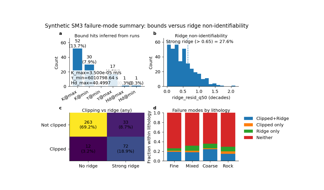
Step 8 - Learn how to read panel (a)

Panel (a) is the bound-hit summary.

Each bar answers:

• how many runs sat exactly at the inferred minimum or maximum,

• and what fraction of all runs that count represents.

This panel is useful because clipping is often invisible if you only inspect scatter plots. A fitted value on the boundary can look innocent unless you count how often it happens.

If one bar is very large, it usually means the optimization is pushing that parameter to the edge of the explored feasible space.

Step 9 - Learn how to read panel (b)

Panel (b) shows the distribution of ridge residuals.

The dashed line is the threshold used to define:

strong ridge

If many runs lie to the right of that line, the model family is telling you that a substantial portion of the experiment space suffers from non-identifiability along the ridge direction.

This panel is therefore not about “good” or “bad” runs in the ordinary predictive sense. It is about whether the inverse problem remains structurally ambiguous.

Step 10 - Learn how to read panel (c)

Panel (c) is the most diagnostic panel on the page.

It cross-tabulates the two failure modes:

• clipped vs not clipped

• strong ridge vs no strong ridge

This is important because it tells you whether the two failure modes are mostly separate or mostly overlapping.

A useful interpretation pattern is:

• top-left: no clipping and no strong ridge -> the safest region

• top-right: no clipping but strong ridge -> not boundary-driven, but still weakly identifiable

• bottom-left: clipped without strong ridge -> a boundary problem more than a ridge problem

• bottom-right: clipped and strong ridge -> the most problematic regime

Step 11 - Learn how to read panel (d)

Panel (d) summarizes the fractions of the four categories.

If lith_idx is absent, the panel shows one overall fraction bar for each category.

If lith_idx is present, as in this lesson, the panel becomes more informative: it shows stacked fractions within each lithology.

That helps answer:

• which lithologies are more vulnerable to clipping?

• which lithologies are more prone to ridge ambiguity?

• and whether the dominant failure mode changes by material type.

Step 12 - Practical takeaway

This figure is useful because it separates two distinct reasons for poor identifiability:

• pushing into bounds,

• sliding along a ridge.

Those are different scientific problems and usually call for different remedies.

For example:

• heavy clipping suggests revisiting bounds, priors, or search ranges,

• strong ridge behaviour suggests revisiting the closure design, the experiment structure, or the identifiability regime.

That is why this figure belongs next to the main SM3 identifiability figure: together they explain both recovery and failure mode.

Command-line version

The same figure can be produced from the command line.

The real script supports:

• --csv for the SM3 runs summary table,

• optional filtering through --only-identify and --nx-min,

• --use with any or primary,

• --ridge-thr and --rtol,

• --paper-format,

• --out-json and --out-csv,

• and the shared plotting text options, including --show-panel-labels for this specific script.

Legacy dispatcher:

python -m scripts plot-sm3-bounds-ridge-summary \
  --csv results/sm3_synth_1d/sm3_synth_runs.csv \
  --use any \
  --ridge-thr 2.0 \
  --out sm3-clip-vs-ridge

Restrict to one identify mode:

python -m scripts plot-sm3-bounds-ridge-summary \
  --csv results/sm3_synth_1d/sm3_synth_runs.csv \
  --only-identify both \
  --nx-min 21 \
  --use primary \
  --paper-format \
  --out sm3-clip-vs-ridge-both

Modern CLI:

geoprior plot sm3-bounds-ridge-summary \
  --csv results/sm3_synth_1d/sm3_synth_runs.csv \
  --use any \
  --out sm3-clip-vs-ridge

The gallery page teaches the figure. The command line reproduces it in a workflow.