
Note
Go to the end to download the full example code.
Quantile recalibration with calibrate_forecasts#
This lesson teaches how to use
geoprior.utils.calibrate.calibrate_forecasts()
to recalibrate individual quantile forecast columns.
Why this page matters#
The earlier uncertainty lessons focused on interval behavior:
widening or shrinking full intervals,
comparing coverage against sharpness,
calibrating exceedance probabilities.
But sometimes the user wants something more specific:
Can we recalibrate each forecast quantile itself?
That is the role of calibrate_forecasts.
What the real function does#
The active implementation in calibrate.py takes a DataFrame that
already contains quantile columns such as:
subsidence_q10subsidence_q50subsidence_q90
plus an observed continuous target column such as
subsidence_actual.
For each quantile level q, it builds a binary target:
then fits either:
isotonic regression, or
logistic calibration,
to approximate the calibrated CDF, and finally inverts that CDF
at the nominal quantile level. The result is a new calibrated column
such as calib_subsidence_q10. The function can also recalibrate
separately per group, for example by forecast_step.
A note about the source file#
The current file contains two different functions named
calibrate_forecasts. The later definition is the one that is
actually active at import time, so this page teaches that later,
DataFrame-based quantile recalibration function.
What this lesson teaches#
We will:
build a synthetic evaluation forecast table,
make the raw quantiles systematically biased,
measure quantile calibration before recalibration,
run the real
calibrate_forecastshelper,compare global versus horizon-wise recalibration,
build explanatory plots showing why it is useful.
This page is synthetic so it remains fully executable during the documentation build.
Imports#
We use the real GeoPrior utility that recalibrates quantile columns.
from __future__ import annotations

import numpy as np
import pandas as pd
import matplotlib.pyplot as plt

from geoprior.utils.calibrate import calibrate_forecasts
Step 1 - Build a compact synthetic evaluation table#
We create one long-format evaluation table with:
sample_idxforecast_stepcoord_tcoord_x,coord_yraw quantile columns
subsidence_actual
The synthetic design is deliberate:
the median forecast is slightly biased high,
the quantile spread is too narrow at longer horizons,
calibration therefore has something meaningful to fix.
rng = np.random.default_rng(61)

nx = 9
ny = 6
steps = [1, 2, 3]
years = {1: 2024, 2: 2025, 3: 2026}

xv = np.linspace(0.0, 12_000.0, nx)
yv = np.linspace(0.0, 8_000.0, ny)
X, Y = np.meshgrid(xv, yv)

x_flat = X.ravel()
y_flat = Y.ravel()
n_sites = x_flat.size

xn = (x_flat - x_flat.min()) / (x_flat.max() - x_flat.min())
yn = (y_flat - y_flat.min()) / (y_flat.max() - y_flat.min())

hotspot = np.exp(
    -(
        ((xn - 0.72) ** 2) / 0.020
        + ((yn - 0.34) ** 2) / 0.032
    )
)
ridge = 0.52 * np.exp(
    -(
        ((xn - 0.28) ** 2) / 0.030
        + ((yn - 0.74) ** 2) / 0.050
    )
)
gradient = 0.44 * xn + 0.22 * (1.0 - yn)

quantiles = [0.1, 0.3, 0.5, 0.7, 0.9]

# Approximate Gaussian z values for the quantiles we use.
z_map = {
    0.1: -1.2816,
    0.3: -0.5244,
    0.5: 0.0,
    0.7: 0.5244,
    0.9: 1.2816,
}

rows: list[dict[str, float | int]] = []

for step in steps:
    scale = {1: 1.00, 2: 1.18, 3: 1.42}[step]

    mu_true = (
        2.2
        + 1.45 * gradient
        + 2.05 * hotspot
        + 0.95 * ridge
    ) * scale

    sigma_true = (
        0.26
        + 0.08 * xn
        + 0.04 * hotspot
        + 0.04 * step
    )

    actual = mu_true + rng.normal(0.0, sigma_true, size=n_sites)

    # Raw forecast is biased and under-dispersed, especially later.
    mu_raw = mu_true + 0.08 * step
    sigma_raw = sigma_true * {1: 0.95, 2: 0.80, 3: 0.68}[step]

    for i in range(n_sites):
        row = {
            "sample_idx": i,
            "forecast_step": step,
            "coord_t": years[step],
            "coord_x": float(x_flat[i]),
            "coord_y": float(y_flat[i]),
            "subsidence_actual": float(actual[i]),
        }

        for q in quantiles:
            col = f"subsidence_q{int(q * 100)}"
            row[col] = float(mu_raw[i] + z_map[q] * sigma_raw[i])

        rows.append(row)

df = pd.DataFrame(rows)

print("Evaluation table shape:", df.shape)
print("")
print(df.head(8).to_string(index=False))
Evaluation table shape: (162, 11)

 sample_idx  forecast_step  coord_t    coord_x  coord_y  subsidence_actual  subsidence_q10  subsidence_q30  subsidence_q50  subsidence_q70  subsidence_q90
          0              1     2024     0.0000   0.0000             2.3490          2.2337          2.4495          2.5990          2.7485          2.9643
          1              1     2024  1500.0000   0.0000             2.2712          2.3013          2.5243          2.6788          2.8332          3.0562
          2              1     2024  3000.0000   0.0000             3.0184          2.3689          2.5991          2.7585          2.9179          3.1481
          3              1     2024  4500.0000   0.0000             2.3857          2.4366          2.6740          2.8384          3.0028          3.2402
          4              1     2024  6000.0000   0.0000             2.2378          2.5088          2.7535          2.9229          3.0923          3.3370
          5              1     2024  7500.0000   0.0000             3.1827          2.6060          2.8583          3.0330          3.2077          3.4599
          6              1     2024  9000.0000   0.0000             3.3541          2.6908          2.9505          3.1304          3.3102          3.5699
          7              1     2024 10500.0000   0.0000             2.7424          2.7230          2.9894          3.1739          3.3584          3.6248
Step 2 - Define a small quantile calibration diagnostic#
A quantile forecast is well calibrated when:
So for each quantile column, we compare:
nominal quantile level alpha,
empirical frequency of
actual <= q_alpha.
If the empirical frequency is below alpha, the quantile is too low. If it is above alpha, the quantile is too high.
def quantile_reliability_table(
    data: pd.DataFrame,
    *,
    prefix: str = "subsidence",
    actual_col: str = "subsidence_actual",
    quantile_levels: list[float] | tuple[float, ...] = (0.1, 0.3, 0.5, 0.7, 0.9),
    calibrated_prefix: str | None = None,
) -> pd.DataFrame:
    rows = []

    y_true = data[actual_col].to_numpy(float)

    for q in quantile_levels:
        qint = int(q * 100)
        if calibrated_prefix is None:
            col = f"{prefix}_q{qint}"
        else:
            col = f"{calibrated_prefix}_{prefix}_q{qint}"

        qhat = data[col].to_numpy(float)
        empirical = float(np.mean(y_true <= qhat))

        rows.append(
            {
                "quantile": float(q),
                "empirical_cdf": empirical,
                "gap": empirical - float(q),
            }
        )

    return pd.DataFrame(rows)


raw_rel = quantile_reliability_table(df)
print("")
print("Raw quantile calibration")
print(raw_rel.to_string(index=False))
Raw quantile calibration
 quantile  empirical_cdf    gap
   0.1000         0.2469 0.1469
   0.3000         0.4877 0.1877
   0.5000         0.6667 0.1667
   0.7000         0.7716 0.0716
   0.9000         0.9506 0.0506
Interpretation#
A perfectly calibrated quantile family would have:
q10 -> empirical_cdf close to 0.10
q50 -> empirical_cdf close to 0.50
q90 -> empirical_cdf close to 0.90
In our synthetic raw forecast, later horizons are intentionally under-dispersed, so the tails should be miscalibrated.
Step 3 - Run the real quantile recalibration helper globally#
We now call the active calibrate_forecasts function.
Important settings:
df: the evaluation DataFrame itself;quantiles: nominal levels expressed as floats in (0, 1);q_prefix="subsidence": tells the helper where to find the raw columns;actual_col="subsidence_actual": observed target;method="isotonic": monotonic non-parametric calibration;out_prefix="calib": output columns likecalib_subsidence_q10.
The function fits a calibration model at each quantile and appends the recalibrated quantile columns to the returned DataFrame.
df_cal_global = calibrate_forecasts(
    df=df,
    quantiles=quantiles,
    q_prefix="subsidence",
    actual_col="subsidence_actual",
    method="isotonic",
    out_prefix="calib",
    grid_mode="range",
    grid_size=1201,
)

print("")
print("Columns after global recalibration")
print(df_cal_global.columns.tolist())

print("")
print(df_cal_global.head(6).to_string(index=False))
Columns after global recalibration
['sample_idx', 'forecast_step', 'coord_t', 'coord_x', 'coord_y', 'subsidence_actual', 'subsidence_q10', 'subsidence_q30', 'subsidence_q50', 'subsidence_q70', 'subsidence_q90', 'calib_subsidence_q10', 'calib_subsidence_q30', 'calib_subsidence_q50', 'calib_subsidence_q70', 'calib_subsidence_q90']

 sample_idx  forecast_step  coord_t   coord_x  coord_y  subsidence_actual  subsidence_q10  subsidence_q30  subsidence_q50  subsidence_q70  subsidence_q90  calib_subsidence_q10  calib_subsidence_q30  calib_subsidence_q50  calib_subsidence_q70  calib_subsidence_q90
          0              1     2024    0.0000   0.0000             2.3490          2.2337          2.4495          2.5990          2.7485          2.9643                1.9241                2.1399                2.2894                3.4813                2.9321
          1              1     2024 1500.0000   0.0000             2.2712          2.3013          2.5243          2.6788          2.8332          3.0562                1.9241                2.1399                2.2894                3.4813                2.9321
          2              1     2024 3000.0000   0.0000             3.0184          2.3689          2.5991          2.7585          2.9179          3.1481                1.9241                2.1399                2.2894                3.4813                2.9321
          3              1     2024 4500.0000   0.0000             2.3857          2.4366          2.6740          2.8384          3.0028          3.2402                1.9241                2.1399                2.2894                3.4813                2.9321
          4              1     2024 6000.0000   0.0000             2.2378          2.5088          2.7535          2.9229          3.0923          3.3370                1.9241                2.1399                2.2894                3.4813                2.9321
          5              1     2024 7500.0000   0.0000             3.1827          2.6060          2.8583          3.0330          3.2077          3.4599                1.9241                2.1399                2.2894                3.4813                2.9321
Step 4 - Measure calibration after global recalibration#
We compute the same quantile reliability table again, now using the recalibrated columns.
cal_rel_global = quantile_reliability_table(
    df_cal_global,
    calibrated_prefix="calib",
)

print("")
print("Globally recalibrated quantiles")
print(cal_rel_global.to_string(index=False))
Globally recalibrated quantiles
 quantile  empirical_cdf     gap
   0.1000         0.0123 -0.0877
   0.3000         0.0123 -0.2877
   0.5000         0.0494 -0.4506
   0.7000         0.5926 -0.1074
   0.9000         0.2531 -0.6469
Step 5 - Run horizon-wise recalibration#
The helper can recalibrate separately per group.
This is important because forecast errors often change with horizon. A single global recalibration may hide that structure.
Here we calibrate separately by forecast_step.
df_cal_by_step = calibrate_forecasts(
    df=df,
    quantiles=quantiles,
    q_prefix="subsidence",
    actual_col="subsidence_actual",
    method="isotonic",
    out_prefix="stepcal",
    grid_mode="range",
    grid_size=1201,
    group_by="forecast_step",
)

print("")
print("Grouped recalibration columns")
print(
    [c for c in df_cal_by_step.columns if c.startswith("stepcal_")]
)
Grouped recalibration columns
['stepcal_subsidence_q10', 'stepcal_subsidence_q30', 'stepcal_subsidence_q50', 'stepcal_subsidence_q70', 'stepcal_subsidence_q90']
Step 6 - Compare global versus horizon-wise reliability#
For grouped recalibration, we summarize the reliability by step and then average the absolute gap from the nominal quantiles.
def mean_abs_gap_by_step(
    data: pd.DataFrame,
    *,
    calibrated_prefix: str | None = None,
) -> pd.DataFrame:
    rows = []
    for step, g in data.groupby("forecast_step", sort=True):
        rel = quantile_reliability_table(
            g,
            calibrated_prefix=calibrated_prefix,
        )
        rows.append(
            {
                "forecast_step": int(step),
                "mean_abs_gap": float(np.mean(np.abs(rel["gap"]))),
            }
        )
    return pd.DataFrame(rows)


gap_raw = mean_abs_gap_by_step(df)
gap_global = mean_abs_gap_by_step(
    df_cal_global,
    calibrated_prefix="calib",
)
gap_group = mean_abs_gap_by_step(
    df_cal_by_step,
    calibrated_prefix="stepcal",
)

df_gap_compare = (
    gap_raw.rename(columns={"mean_abs_gap": "raw_gap"})
    .merge(
        gap_global.rename(columns={"mean_abs_gap": "global_gap"}),
        on="forecast_step",
    )
    .merge(
        gap_group.rename(columns={"mean_abs_gap": "group_gap"}),
        on="forecast_step",
    )
)

print("")
print("Mean absolute quantile-calibration gap by step")
print(df_gap_compare.to_string(index=False))
Mean absolute quantile-calibration gap by step
 forecast_step  raw_gap  global_gap  group_gap
             1   0.0778      0.2459     0.2815
             2   0.0815      0.3407     0.1074
             3   0.2148      0.4519     0.2407
Why grouped recalibration matters#
If calibration error changes across the horizon, grouped recalibration is often more appropriate than fitting one single global transform for every step.
Step 7 - Plot quantile calibration before and after#
This is the most important figure of the lesson.
A quantile calibration curve should ideally follow the diagonal:
x-axis: nominal quantile level
y-axis: empirical frequency of
actual <= q_alpha
fig, ax = plt.subplots(figsize=(6.8, 6.2))

ax.plot([0, 1], [0, 1], linestyle="--", linewidth=1.5)

ax.plot(
    raw_rel["quantile"],
    raw_rel["empirical_cdf"],
    marker="o",
    label="Raw",
)
ax.plot(
    cal_rel_global["quantile"],
    cal_rel_global["empirical_cdf"],
    marker="s",
    label="Global recalibration",
)

# Build one average grouped curve for display
group_rows = []
for q in quantiles:
    vals = []
    for _, g in df_cal_by_step.groupby("forecast_step", sort=True):
        rel = quantile_reliability_table(
            g,
            quantile_levels=[q],
            calibrated_prefix="stepcal",
        )
        vals.append(float(rel["empirical_cdf"].iloc[0]))
    group_rows.append(
        {
            "quantile": q,
            "empirical_cdf": float(np.mean(vals)),
        }
    )

group_curve = pd.DataFrame(group_rows)

ax.plot(
    group_curve["quantile"],
    group_curve["empirical_cdf"],
    marker="^",
    label="Grouped recalibration",
)

ax.set_xlim(0, 1)
ax.set_ylim(0, 1)
ax.set_aspect("equal", adjustable="box")
ax.set_xlabel("Nominal quantile level")
ax.set_ylabel("Empirical frequency")
ax.set_title("Quantile calibration curve")
ax.grid(True, linestyle=":", alpha=0.6)
ax.legend()

plt.tight_layout()
plt.show()
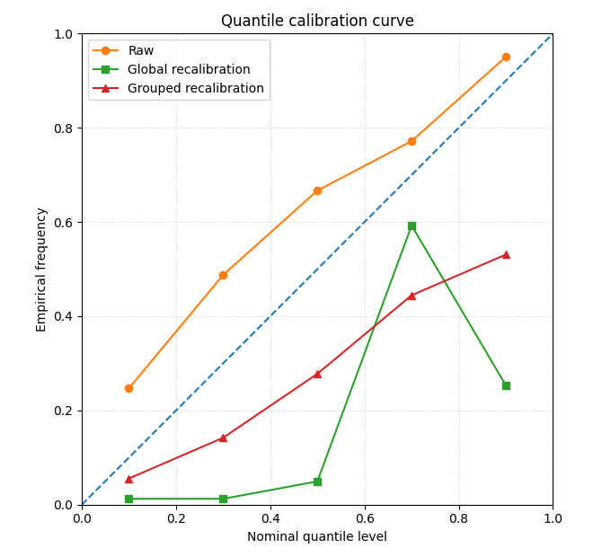
How to read this figure#
The diagonal is the target.
Curves below the diagonal indicate quantiles that are too low: the truth falls below them less often than claimed.
Curves above the diagonal indicate quantiles that are too high: the truth falls below them more often than claimed.
A successful recalibration moves the curve closer to the diagonal.
Step 8 - Plot calibration improvement by horizon#
This second figure answers:
where does recalibration help most?
We compare the mean absolute quantile-calibration gap by step.
fig, ax = plt.subplots(figsize=(7.2, 4.6))

ax.plot(
    df_gap_compare["forecast_step"],
    df_gap_compare["raw_gap"],
    marker="o",
    label="Raw",
)
ax.plot(
    df_gap_compare["forecast_step"],
    df_gap_compare["global_gap"],
    marker="s",
    label="Global recalibration",
)
ax.plot(
    df_gap_compare["forecast_step"],
    df_gap_compare["group_gap"],
    marker="^",
    label="Grouped recalibration",
)

ax.set_xlabel("Forecast step")
ax.set_ylabel("Mean absolute calibration gap")
ax.set_title("Quantile calibration gap across the horizon")
ax.grid(True, linestyle=":", alpha=0.6)
ax.legend()

plt.tight_layout()
plt.show()
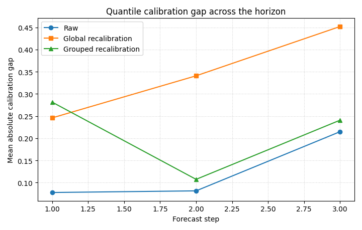
What this panel tells us#
A grouped recalibration often helps most when later horizons behave differently from early ones. This is especially useful in forecast systems where uncertainty grows non-uniformly with lead time.
Step 9 - Inspect how one quantile map changes spatially#
To make the effect more concrete, we inspect the upper quantile q90 at the last horizon step.
This is not a full forecast map page. It is just a compact visual check that recalibration can change the threshold surface itself.
step_to_plot = 3

g_raw = df[df["forecast_step"] == step_to_plot].copy()
g_cal = df_cal_by_step[
    df_cal_by_step["forecast_step"] == step_to_plot
].copy()

fig, axes = plt.subplots(1, 2, figsize=(9.8, 4.1))

sc0 = axes[0].scatter(
    g_raw["coord_x"],
    g_raw["coord_y"],
    c=g_raw["subsidence_q90"],
    s=32,
)
axes[0].set_title("Raw q90")
axes[0].set_xlabel("coord_x")
axes[0].set_ylabel("coord_y")
axes[0].grid(True, linestyle=":", alpha=0.4)

sc1 = axes[1].scatter(
    g_cal["coord_x"],
    g_cal["coord_y"],
    c=g_cal["stepcal_subsidence_q90"],
    s=32,
)
axes[1].set_title("Grouped calibrated q90")
axes[1].set_xlabel("coord_x")
axes[1].set_ylabel("coord_y")
axes[1].grid(True, linestyle=":", alpha=0.4)

fig.colorbar(sc0, ax=axes[0], shrink=0.85)
fig.colorbar(sc1, ax=axes[1], shrink=0.85)

plt.tight_layout()
plt.show()
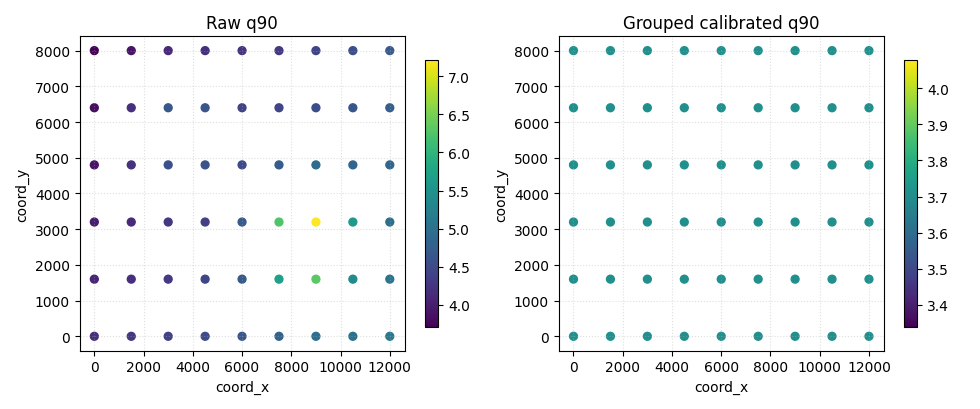
Why this spatial check is useful#
calibrate_forecasts does not only change a score. It changes the
quantile surfaces themselves.
That matters because later uncertainty and risk pages may use these calibrated quantiles directly.
Step 10 - Compare isotonic and logistic modes#
The active helper also supports method="logistic".
We run it once here so the page shows the alternative mode, even though isotonic is often more flexible for monotonic recalibration.
df_cal_log = calibrate_forecasts(
    df=df,
    quantiles=quantiles,
    q_prefix="subsidence",
    actual_col="subsidence_actual",
    method="logistic",
    out_prefix="logcal",
    grid_mode="range",
    grid_size=1201,
)

log_rel = quantile_reliability_table(
    df_cal_log,
    calibrated_prefix="logcal",
)

print("")
print("Logistic recalibration")
print(log_rel.to_string(index=False))
Logistic recalibration
 quantile  empirical_cdf     gap
   0.1000         0.0123 -0.0877
   0.3000         0.0123 -0.2877
   0.5000         0.0494 -0.4506
   0.7000         0.1481 -0.5519
   0.9000         0.1543 -0.7457
Interpretation#
Logistic mode is more parametric and smoother, while isotonic mode is more flexible and purely monotonic.
Which one is better depends on:
sample size,
smoothness of the distortion,
and whether the calibration error looks roughly sigmoidal or not.
Final takeaway#
calibrate_forecasts is the uncertainty utility to use when you
want to recalibrate the quantile columns themselves, not only the
overall interval width and not only a binary exceedance probability.
It belongs late in the uncertainty section because it builds on ideas introduced earlier:
interval honesty,
calibration curves,
probability calibration,
and horizon-specific uncertainty behavior.
Total running time of the script: (0 minutes 0.614 seconds)