
Note
Go to the end to download the full example code.
Build a compact forecast-ready panel sample#
This example teaches you how to use GeoPrior’s
forecast-ready-sample build utility.
Unlike the earlier spatial samplers, this builder does not focus on individual rows. It focuses on spatial groups with enough temporal history to support a forecasting window.
Why this matters#
A forecasting demo or smoke test usually needs more than a random subset of rows. It needs a compact panel where each sampled location still has:
stable group identity,
enough years for the lookback window,
enough years for the forecast horizon,
and a spatial footprint that is still representative.
That is exactly what forecast-ready-sample is for.
Imports#
We call the real production entrypoint from the project code.
For the synthetic dataset itself, we reuse the shared spatial-support
helpers from geoprior.scripts.utils rather than generating plain
random points by hand.
from __future__ import annotations

import tempfile
from pathlib import Path

import matplotlib.pyplot as plt
import numpy as np
import pandas as pd

from geoprior.cli.build_forecast_ready_sample import (
    build_forecast_ready_sample_main,
)
from geoprior.scripts import utils as script_utils
Build two synthetic city supports#
We start from the shared SpatialSupportSpec helper so the lesson
stays consistent with the rest of the gallery.
Key parameters#
- city:
Human-readable city label attached to the support.
- center_x, center_y:
Center of the synthetic geographic cloud.
- span_x, span_y:
Half-width and half-height of the support extent.
- nx, ny:
Mesh density before masking.
- jitter_x, jitter_y:
Small perturbations so the support is not a perfect grid.
- footprint:
Synthetic city shape.
- keep_frac:
Fraction of masked points retained.
- seed:
Keeps the support reproducible across documentation builds.
ns_support = script_utils.make_spatial_support(
    script_utils.SpatialSupportSpec(
        city="Nansha",
        center_x=113.52,
        center_y=22.74,
        span_x=0.16,
        span_y=0.11,
        nx=26,
        ny=20,
        jitter_x=0.0013,
        jitter_y=0.0011,
        footprint="nansha_like",
        keep_frac=0.86,
        seed=31,
    )
)

zh_support = script_utils.make_spatial_support(
    script_utils.SpatialSupportSpec(
        city="Zhongshan",
        center_x=113.38,
        center_y=22.53,
        span_x=0.18,
        span_y=0.12,
        nx=27,
        ny=21,
        jitter_x=0.0014,
        jitter_y=0.0011,
        footprint="zhongshan_like",
        keep_frac=0.84,
        seed=47,
    )
)

print("Synthetic support sizes")
print(f" - Nansha   : {ns_support.sample_idx.size:,} points")
print(f" - Zhongshan: {zh_support.sample_idx.size:,} points")
Synthetic support sizes
 - Nansha   : 208 points
 - Zhongshan: 210 points
Build a multi-year synthetic forecasting panel#
forecast-ready-sample expects a regular panel DataFrame. We build
one from the reusable supports with:
a stable point identifier,
longitude and latitude,
yearly observations,
two continuous drivers,
one categorical geology-like class,
and one response-like target.
The synthetic signals are intentionally smooth in space and time so the lesson stays interpretable.
rng = np.random.default_rng(123)
years = list(range(2018, 2025))
frames: list[pd.DataFrame] = []

for support, amp0, drift_x, drift_y in [
    (ns_support, 4.9, 0.12, 0.08),
    (zh_support, 5.6, 0.08, 0.10),
]:
    base_subs = script_utils.make_spatial_field(
        support,
        amplitude=amp0,
        drift_x=drift_x,
        drift_y=drift_y,
        phase=0.22,
        hotspot_weight=0.92,
        secondary_weight=0.56,
        ridge_weight=0.18,
        wave_weight=0.14,
        local_weight=0.08,
    )

    base_scale = script_utils.make_spatial_scale(
        support,
        base=0.24,
        x_weight=0.08,
        hotspot_weight=0.05,
    )

    for year in years:
        step = year - years[0]

        frame = support.to_frame().rename(
            columns={
                "coord_x": "longitude",
                "coord_y": "latitude",
            }
        )
        frame["year"] = int(year)
        frame["point_id"] = [
            f"{support.city}_{idx:04d}"
            for idx in frame["sample_idx"].to_numpy(int)
        ]

        # Smooth categorical structure across the city footprint.
        frame["lithology_class"] = np.where(
            frame["y_norm"] > 0.63,
            "Clay",
            np.where(frame["x_norm"] > 0.58, "Fill", "Sand"),
        )

        # Compact but useful synthetic drivers.
        frame["rainfall_mm"] = (
            1180
            + 52 * step
            + 42 * frame["y_norm"]
            + rng.normal(0.0, 11.0, len(frame))
        )
        frame["gwl_depth_bgs_m"] = (
            2.2
            + 0.20 * step
            + 1.1 * (1.0 - frame["y_norm"])
            + rng.normal(0.0, 0.08, len(frame))
        )
        frame["normalized_urban_load_proxy"] = np.clip(
            0.18
            + 0.42 * frame["x_norm"]
            + 0.25 * frame["y_norm"]
            + rng.normal(0.0, 0.03, len(frame)),
            0.0,
            1.0,
        )

        # Evolve the response through time while preserving the same
        # broad geography. Later years become slightly more intense.
        evolved = script_utils.evolve_spatial_field(
            support,
            base_field=base_subs,
            step=step,
            growth=1.0 + 0.07 * step,
        )
        noise = rng.normal(0.0, base_scale * (0.70 + 0.04 * step))
        frame["subsidence_mm"] = (
            evolved
            + 0.40 * frame["normalized_urban_load_proxy"]
            + 0.10 * frame["gwl_depth_bgs_m"]
            + noise
        )

        frames.append(frame)

full_df = pd.concat(frames, ignore_index=True)

print("")
print("Synthetic full panel")
print(full_df.head(8).to_string(index=False))
Synthetic full panel
 sample_idx  longitude  latitude  x_norm  y_norm   city  year    point_id lithology_class  rainfall_mm  gwl_depth_bgs_m  normalized_urban_load_proxy  subsidence_mm
          0   113.4760   22.6659  0.3656  0.1716 Nansha  2018 Nansha_0000            Sand    1176.3274           2.9243                       0.3520         1.5043
          1   113.4885   22.6645  0.4040  0.1653 Nansha  2018 Nansha_0001            Sand    1182.8972           3.2086                       0.4196         0.6527
          2   113.4987   22.6654  0.4350  0.1697 Nansha  2018 Nansha_0002            Sand    1201.2936           3.3237                       0.3848         0.6798
          3   113.5122   22.6637  0.4765  0.1618 Nansha  2018 Nansha_0003            Sand    1188.9275           3.1583                       0.3849         0.3992
          4   113.5255   22.6648  0.5169  0.1669 Nansha  2018 Nansha_0004            Sand    1197.1317           3.1352                       0.4196         0.6210
          5   113.5401   22.6629  0.5615  0.1582 Nansha  2018 Nansha_0005            Sand    1192.9923           3.1819                       0.4392         0.4430
          6   113.5524   22.6640  0.5992  0.1634 Nansha  2018 Nansha_0006            Fill    1179.8620           3.1785                       0.4691         0.2389
          7   113.5652   22.6645  0.6383  0.1656 Nansha  2018 Nansha_0007            Fill    1192.9163           3.1286                       0.4760         0.6290
Deliberately make some groups ineligible#
The builder is interesting because it filters groups that do not keep enough temporal history.
To make that behavior visible, we intentionally damage part of the synthetic panel by dropping years for some point IDs. These damaged groups will fail the required window length later.
base_points = (
    full_df.loc[:, ["point_id", "city"]]
    .drop_duplicates()
    .reset_index(drop=True)
)

broken_ids: list[str] = []

for city in ["Nansha", "Zhongshan"]:
    city_ids = base_points.loc[
        base_points["city"] == city, "point_id"
    ].to_numpy()

    n_break = max(10, int(0.14 * len(city_ids)))
    chosen = rng.choice(city_ids, size=n_break, replace=False)
    broken_ids.extend(chosen.tolist())

full_df = full_df.loc[
    ~(
        full_df["point_id"].isin(broken_ids)
        & full_df["year"].isin([2019, 2021, 2023])
    )
].copy()
Compute a simple eligibility summary before building#
The real builder checks whether each group has enough years and, optionally, enough consecutive years. We reproduce a small summary here so users can see what the builder will filter out.
def _longest_consecutive_run(values: list[int] | np.ndarray) -> int:
    years_arr = np.asarray(sorted(set(int(v) for v in values)), dtype=int)
    if years_arr.size == 0:
        return 0
    if years_arr.size == 1:
        return 1

    longest = 1
    current = 1
    for diff in np.diff(years_arr):
        if int(diff) == 1:
            current += 1
            longest = max(longest, current)
        else:
            current = 1
    return int(longest)


stats_rows: list[dict[str, object]] = []
for point_id, g in full_df.groupby("point_id", sort=False):
    years_i = sorted(pd.unique(g["year"]))
    stats_rows.append(
        {
            "point_id": point_id,
            "city": g["city"].iloc[0],
            "n_years": int(len(years_i)),
            "longest_run": _longest_consecutive_run(years_i),
            "eligible": (
                len(years_i) >= 5
                and _longest_consecutive_run(years_i) >= 5
            ),
        }
    )

eligibility = pd.DataFrame(stats_rows)

elig_summary = (
    eligibility.groupby(["city", "eligible"])
    .size()
    .rename("n_groups")
    .reset_index()
)

print("")
print("Eligibility summary before building")
print(elig_summary.to_string(index=False))
Eligibility summary before building
     city  eligible  n_groups
   Nansha     False        29
   Nansha      True       179
Zhongshan     False        29
Zhongshan      True       181
Write one input file per city#
The shared build-reader utilities accept one or many files, so the lesson demonstrates the multi-file workflow directly.
tmp_dir = Path(
    tempfile.mkdtemp(prefix="gp_sg_forecast_ready_sample_")
)

ns_csv = tmp_dir / "nansha_panel.csv"
zh_csv = tmp_dir / "zhongshan_panel.csv"
out_csv = tmp_dir / "forecast_ready_demo_panel.csv"

full_df.loc[full_df["city"] == "Nansha"].to_csv(
    ns_csv,
    index=False,
)
full_df.loc[full_df["city"] == "Zhongshan"].to_csv(
    zh_csv,
    index=False,
)

print("")
print("Input files")
print(" -", ns_csv.name)
print(" -", zh_csv.name)
Input files
 - nansha_panel.csv
 - zhongshan_panel.csv
Run the real forecast-ready builder#
We now call the production CLI entrypoint exactly as a user would.
Key choices in this lesson#
- –group-cols point_id:
treat each point ID as one temporal group.
- –stratify-by city lithology_class:
keep the sampled groups representative by city and geology.
- –time-steps 3 and –forecast-horizon 2:
require a 5-year usable window.
- –keep-years 5 and –year-mode latest:
once groups are sampled, keep the latest 5 years per group.
- –require-consecutive:
reject groups whose time history is too fragmented.
build_forecast_ready_sample_main(
    [
        str(ns_csv),
        str(zh_csv),
        "--out",
        str(out_csv),
        "--time-col",
        "year",
        "--spatial-cols",
        "longitude",
        "latitude",
        "--group-cols",
        "point_id",
        "--stratify-by",
        "city",
        "lithology_class",
        "--spatial-bins",
        "10",
        "8",
        "--sample-size",
        "110",
        "--time-steps",
        "3",
        "--forecast-horizon",
        "2",
        "--keep-years",
        "5",
        "--year-mode",
        "latest",
        "--method",
        "abs",
        "--min-groups",
        "25",
        "--require-consecutive",
        "--sort-output",
        "--random-state",
        "42",
        "--verbose",
        "1",
    ],
    prog="forecast-ready-sample",
)
[INFO] Built forecast-ready sample: 575 rows, 115 groups, min_required_years=5, keep_years=5

[OK] forecast-ready sample written
  path   : /tmp/gp_sg_forecast_ready_sample_qguylhdy/forecast_ready_demo_panel.csv
  rows   : 575
  groups : 115
  window : T=3, H=2
Read the compact output panel back in#
The builder returns a smaller panel that is still ready for forecasting demos and quick tests.
sampled_df = pd.read_csv(out_csv)

print("")
print("Sampled panel")
print(sampled_df.head(10).to_string(index=False))
Sampled panel
 sample_idx  longitude  latitude  x_norm  y_norm   city  year    point_id lithology_class  rainfall_mm  gwl_depth_bgs_m  normalized_urban_load_proxy  subsidence_mm
          4   113.5255   22.6648  0.5169  0.1669 Nansha  2020 Nansha_0004            Sand    1303.4826           3.5888                       0.4786         0.5845
          4   113.5255   22.6648  0.5169  0.1669 Nansha  2021 Nansha_0004            Sand    1332.8251           3.7012                       0.4008         1.4910
          4   113.5255   22.6648  0.5169  0.1669 Nansha  2022 Nansha_0004            Sand    1391.8147           3.9097                       0.4514         2.4410
          4   113.5255   22.6648  0.5169  0.1669 Nansha  2023 Nansha_0004            Sand    1476.4561           4.1640                       0.4509         1.9786
          4   113.5255   22.6648  0.5169  0.1669 Nansha  2024 Nansha_0004            Sand    1494.1083           4.5073                       0.4470         0.8524
          6   113.5524   22.6640  0.5992  0.1634 Nansha  2020 Nansha_0006            Fill    1284.6474           3.5927                       0.4533         0.9449
          6   113.5524   22.6640  0.5992  0.1634 Nansha  2021 Nansha_0006            Fill    1344.8097           3.6212                       0.4621         1.7066
          6   113.5524   22.6640  0.5992  0.1634 Nansha  2022 Nansha_0006            Fill    1406.0549           3.6822                       0.5296         1.7746
          6   113.5524   22.6640  0.5992  0.1634 Nansha  2023 Nansha_0006            Fill    1456.1462           4.0030                       0.4621         1.6196
          6   113.5524   22.6640  0.5992  0.1634 Nansha  2024 Nansha_0006            Fill    1492.3063           4.2288                       0.4860         1.4483
Summarize the sampled groups#
We compute a few compact checks:
how many sampled groups each city kept,
how many rows per year remain,
and whether the sampled groups really have the requested 5 years.
sampled_group_summary = (
    sampled_df.groupby("point_id")
    .agg(
        city=("city", "first"),
        n_rows=("year", "size"),
        min_year=("year", "min"),
        max_year=("year", "max"),
    )
    .reset_index()
)

sampled_city_counts = (
    sampled_group_summary.groupby("city")
    .size()
    .rename("sampled_groups")
    .reset_index()
)

year_counts = (
    sampled_df.groupby("year")
    .size()
    .rename("rows")
    .reset_index()
)

print("")
print("Sampled groups by city")
print(sampled_city_counts.to_string(index=False))

print("")
print("Rows by year in the compact panel")
print(year_counts.to_string(index=False))

print("")
print("Per-group row counts in the compact panel")
print(
    sampled_group_summary["n_rows"]
    .value_counts()
    .sort_index()
    .rename_axis("rows_per_group")
    .reset_index(name="n_groups")
    .to_string(index=False)
)
Sampled groups by city
     city  sampled_groups
   Nansha              56
Zhongshan              59

Rows by year in the compact panel
 year  rows
 2020   115
 2021   115
 2022   115
 2023   115
 2024   115

Per-group row counts in the compact panel
 rows_per_group  n_groups
              5       115
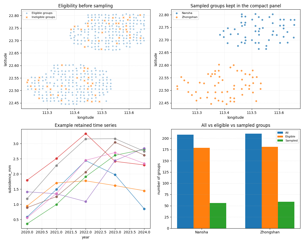
Build one compact visual preview#
This preview is a teaching aid for the gallery page.
- Top-left:
all groups, highlighting the ineligible ones.
- Top-right:
sampled groups after the builder.
- Bottom-left:
several retained time series, proving the panel nature is kept.
- Bottom-right:
all / eligible / sampled group counts by city.
full_points = full_df.groupby("point_id", as_index=False).first()
full_points = full_points.merge(
    eligibility.loc[:, ["point_id", "eligible"]],
    on="point_id",
    how="left",
)

sampled_points = sampled_df.groupby("point_id", as_index=False).first()

count_summary = (
    full_points.groupby("city")
    .size()
    .rename("all_groups")
    .reset_index()
    .merge(
        full_points.loc[full_points["eligible"]]
        .groupby("city")
        .size()
        .rename("eligible_groups")
        .reset_index(),
        on="city",
        how="left",
    )
    .merge(sampled_city_counts, on="city", how="left")
    .fillna(0)
)

count_summary[["eligible_groups", "sampled_groups"]] = (
    count_summary[["eligible_groups", "sampled_groups"]]
    .astype(int)
)

fig, axes = plt.subplots(2, 2, figsize=(12.0, 9.6))

# All groups, with ineligible ones highlighted.
ax = axes[0, 0]
sub_ok = full_points.loc[full_points["eligible"]]
sub_bad = full_points.loc[~full_points["eligible"]]
ax.scatter(
    sub_ok["longitude"],
    sub_ok["latitude"],
    s=10,
    alpha=0.35,
    label="Eligible groups",
)
ax.scatter(
    sub_bad["longitude"],
    sub_bad["latitude"],
    s=18,
    alpha=0.80,
    marker="x",
    label="Ineligible groups",
)
ax.set_title("Eligibility before sampling")
ax.set_xlabel("longitude")
ax.set_ylabel("latitude")
ax.legend(fontsize=8)
ax.grid(True, linestyle=":", alpha=0.45)

# Sampled groups.
ax = axes[0, 1]
for city in ["Nansha", "Zhongshan"]:
    sub = sampled_points.loc[sampled_points["city"] == city]
    ax.scatter(
        sub["longitude"],
        sub["latitude"],
        s=16,
        alpha=0.70,
        label=city,
    )
ax.set_title("Sampled groups kept in the compact panel")
ax.set_xlabel("longitude")
ax.set_ylabel("latitude")
ax.legend(fontsize=8)
ax.grid(True, linestyle=":", alpha=0.45)

# Several retained trajectories.
ax = axes[1, 0]
show_ids = sampled_group_summary["point_id"].head(8).tolist()
for point_id in show_ids:
    sub = sampled_df.loc[
        sampled_df["point_id"] == point_id
    ].sort_values("year")
    ax.plot(
        sub["year"],
        sub["subsidence_mm"],
        marker="o",
        linewidth=1.2,
        alpha=0.85,
    )
ax.set_title("Example retained time series")
ax.set_xlabel("year")
ax.set_ylabel("subsidence_mm")
ax.grid(True, linestyle=":", alpha=0.45)

# Group counts by city.
ax = axes[1, 1]
x = np.arange(len(count_summary))
width = 0.24
ax.bar(x - width, count_summary["all_groups"], width, label="All")
ax.bar(
    x,
    count_summary["eligible_groups"],
    width,
    label="Eligible",
)
ax.bar(
    x + width,
    count_summary["sampled_groups"],
    width,
    label="Sampled",
)
ax.set_xticks(x)
ax.set_xticklabels(count_summary["city"])
ax.set_ylabel("number of groups")
ax.set_title("All vs eligible vs sampled groups")
ax.legend(fontsize=8)
ax.grid(True, axis="y", linestyle=":", alpha=0.45)

plt.tight_layout()
Learn how to read the compact panel#
The output is still a regular table, but it now has a different role.
A useful reading order is:
identify the group columns such as
point_idandcity;confirm the time window with
year;inspect the retained drivers and response columns;
only then check whether the compact panel is large enough for the downstream demo or test.
In other words:
the full panel is the large source table,
the compact panel is the reusable forecasting subset.
Learn why the group-wise sampling matters#
A row-wise sample would often break the temporal continuity needed by a forecasting model.
This builder instead:
samples groups spatially,
checks whether each group has enough history,
then reconstructs the full short panel for the selected groups.
That is why it is much safer for smoke tests and gallery demos.
Learn what keep_years changes#
In this lesson we asked for --keep-years 5 and --year-mode
latest.
That means the builder does not keep the full original history. It keeps only the latest five years for each sampled group.
This is often exactly what a compact forecasting demo needs: enough history to build sequences, but not unnecessary older rows.
Practical takeaway#
A good workflow for forecasting demos is:
start from a full multi-year city panel,
build a compact forecast-ready sample,
confirm the sampled groups still have the required years,
inspect a few retained time series,
then use the compact panel for training or documentation demos.
This order keeps the data-preparation logic clear before any model code is introduced.
Command-line version#
The same lesson can be reproduced from the CLI.
Family-specific entry point:
geoprior-build forecast-ready-sample \
nansha_panel.csv zhongshan_panel.csv \
--out demo_panel.csv \
--time-col year \
--spatial-cols longitude latitude \
--group-cols point_id \
--stratify-by city lithology_class \
--spatial-bins 10 8 \
--sample-size 110 \
--time-steps 3 \
--forecast-horizon 2 \
--keep-years 5 \
--year-mode latest \
--require-consecutive
Root dispatcher:
geoprior build forecast-ready-sample \
  nansha_panel.csv zhongshan_panel.csv \
  --out demo_panel.csv \
  --time-steps 3 \
  --forecast-horizon 2 \
  --keep-years 5
The gallery page teaches the builder. The command line reproduces it in a workflow.
Total running time of the script: (0 minutes 0.877 seconds)