
Note
Go to the end to download the full example code.
Inspect a training summary before trusting a Stage-2 run#
This lesson explains how to inspect the Stage-2
training_summary.json artifact.
A training summary is one of the most decision-oriented artifacts in the GeoPrior workflow. It is not just a metric snapshot. It is the compact place where a user can verify:
which run was trained,
which epoch was selected as best,
whether training and validation tell a similar story,
whether physics losses stayed small or started to dominate,
whether interval quality looks plausible,
and whether the run exported the files needed downstream.
The goal of this page is therefore not only to call helper functions. It is to teach how to read the artifact step by step and decide whether the run looks healthy enough for later evaluation, calibration, inference, or export.
from __future__ import annotations

import json
import tempfile
from pathlib import Path
from pprint import pprint

import matplotlib.pyplot as plt
import pandas as pd

from geoprior.utils.inspect import (
    generate_training_summary,
    inspect_training_summary,
    load_training_summary,
    plot_training_best_metrics,
    plot_training_boolean_summary,
    plot_training_final_metrics,
    plot_training_loss_family,
    plot_training_metric_deltas,
    summarize_training_summary,
    training_compile_frame,
    training_env_frame,
    training_hp_frame,
    training_metrics_frame,
    training_paths_frame,
)

pd.set_option("display.max_columns", 30)
pd.set_option("display.width", 108)
pd.set_option("display.max_colwidth", 80)

TRAIN_COLORS = {
    "best": "#2563eb",
    "final": "#0f766e",
    "loss": "#7c3aed",
    "accent": "#d97706",
    "pass": "#16a34a",
    "fail": "#dc2626",
    "ink": "#0f172a",
    "muted": "#64748b",
    "grid": "#cbd5e1",
    "face": "#f8fafc",
}


def _style_axes(ax: plt.Axes, *, facecolor: str = TRAIN_COLORS["face"]) -> None:
    ax.set_facecolor(facecolor)
    ax.set_axisbelow(True)
    ax.grid(True, color=TRAIN_COLORS["grid"], alpha=0.45, linewidth=0.8)
    for side in ("top", "right"):
        ax.spines[side].set_visible(False)
    for side in ("left", "bottom"):
        ax.spines[side].set_color("#94a3b8")
        ax.spines[side].set_linewidth(0.9)
    ax.tick_params(colors=TRAIN_COLORS["ink"], labelsize=9)
    if ax.get_title():
        ax.set_title(ax.get_title(), fontsize=11, fontweight="bold", color=TRAIN_COLORS["ink"], pad=12)
    if ax.get_xlabel():
        ax.set_xlabel(ax.get_xlabel(), fontsize=9.5, color=TRAIN_COLORS["muted"])
    if ax.get_ylabel():
        ax.set_ylabel(ax.get_ylabel(), fontsize=9.5, color=TRAIN_COLORS["muted"])


def _style_bars(ax: plt.Axes, colors: list[str], *, edgecolor: str = TRAIN_COLORS["ink"], linewidth: float = 1.1, alpha: float = 0.95) -> None:
    for idx, patch in enumerate(ax.patches):
        patch.set_facecolor(colors[idx % len(colors)])
        patch.set_edgecolor(edgecolor)
        patch.set_linewidth(linewidth)
        patch.set_alpha(alpha)


def _style_delta_bars(ax: plt.Axes) -> None:
    for patch in ax.patches:
        value = patch.get_width() if patch.get_width() else patch.get_height()
        color = TRAIN_COLORS["final"] if value <= 0 else TRAIN_COLORS["accent"]
        patch.set_facecolor(color)
        patch.set_edgecolor(TRAIN_COLORS["ink"])
        patch.set_linewidth(1.1)
        patch.set_alpha(0.95)


def _style_boolean_bars(ax: plt.Axes) -> None:
    for patch in ax.patches:
        value = patch.get_width() if patch.get_width() else patch.get_height()
        color = TRAIN_COLORS["pass"] if value >= 0.5 else TRAIN_COLORS["fail"]
        patch.set_facecolor(color)
        patch.set_edgecolor(TRAIN_COLORS["ink"])
        patch.set_linewidth(1.1)
        patch.set_alpha(0.95)
Why this artifact matters#
The training summary is one of the best files to inspect immediately after Stage-2 training. It is smaller than a full history log, but still rich enough to answer practical review questions:
Which epoch was chosen as the best checkpoint?
Did validation improve in the same direction as training?
Did the run keep physics terms under control?
Did interval diagnostics such as coverage and sharpness look plausible at the selected checkpoint?
Were the expected model files and logs exported?
In other words, this artifact helps the user decide whether a run is ready for deeper evaluation or whether it should be revisited before spending more time downstream.
Create a realistic demo training summary#
For documentation pages, we want a stable artifact that behaves like a real training summary without rerunning a training job. The generation helper was designed exactly for that purpose.
Here we create a realistic summary with:
a clear best epoch,
train and validation metrics,
compile settings,
initialization hyperparameters,
and a realistic output-path bundle.
out_dir = Path(tempfile.mkdtemp(prefix="gp_training_summary_"))
summary_path = out_dir / "nansha_training_summary.json"

generate_training_summary(
    output_path=summary_path,
    city="nansha",
    model="GeoPriorSubsNet",
    horizon=3,
    best_epoch=17,
    timestamp="2026-03-29 09:18:44",
    optimizer="Adam",
    learning_rate=8e-4,
    time_steps=5,
    pde_mode="on",
    offset_mode="mul",
    coords_normalized=True,
    coord_ranges={"t": 7.0, "x": 44447.0, "y": 39275.0},
    run_dir=(
        "results/nansha_GeoPriorSubsNet_stage1/"
        "train_20260329-091844"
    ),
)

print("Written training-summary file")
print(f" - {summary_path}")
Written training-summary file
 - /tmp/gp_training_summary_ce1z2xtr/nansha_training_summary.json
Load the artifact with the real reader#
Even in a lesson, it is worth using the same entry point a real workflow would use. That keeps the example close to a user’s actual inspection path.
summary_record = load_training_summary(summary_path)

print("\nArtifact header")
pprint(
    {
        "kind": summary_record.kind,
        "stage": summary_record.stage,
        "city": summary_record.city,
        "model": summary_record.model,
        "path": str(summary_record.path),
    }
)
Artifact header
{'city': 'nansha',
 'kind': 'training_summary',
 'model': 'GeoPriorSubsNet',
 'path': '/tmp/gp_training_summary_ce1z2xtr/nansha_training_summary.json',
 'stage': None}
Start with the compact semantic summary#
Before reading every nested section, start from the compact semantic summary.
This is the first decision checkpoint because it condenses the artifact into three practical layers:
a short identity block,
the core metrics that matter most for review,
and boolean checks that answer whether the run looks complete.
When users inspect many runs, this summary is often the fastest way to decide which run deserves deeper analysis.
summary = summarize_training_summary(summary_record)

print("\nCompact summary")
print(json.dumps(summary, indent=2))
Compact summary
{
  "brief": {
    "kind": "training_summary",
    "city": "nansha",
    "model": "GeoPriorSubsNet",
    "timestamp": "2026-03-29 09:18:44",
    "horizon": 3,
    "best_epoch": 17
  },
  "core_metrics": {
    "best_train_loss": 0.0568,
    "best_val_loss": 0.049416,
    "final_train_loss": 0.05445,
    "final_val_loss": 0.04951,
    "best_train_subs_mae_q50": 0.0101,
    "best_val_subs_mae_q50": 0.008787,
    "best_train_gwl_mae_q50": 0.24,
    "best_val_gwl_mae_q50": 0.20879999999999999,
    "best_val_coverage80": 0.8160000000000001,
    "best_val_sharpness80": 0.026709,
    "delta_final_minus_best_val_loss": 9.399999999999686e-05
  },
  "compile": {
    "optimizer": "Adam",
    "learning_rate": 0.0008,
    "lambda_offset": 1.0,
    "loss_weight_keys": [
      "subs_pred",
      "gwl_pred"
    ]
  },
  "checks": {
    "has_best_metrics": true,
    "has_final_metrics": true,
    "has_validation_metrics": true,
    "has_physics_metrics": true,
    "best_epoch_is_positive": true,
    "lambda_offset_stable": true,
    "quantiles_defined": true,
    "has_scaling_kwargs": true,
    "has_saved_model_paths": true,
    "has_optimizer": true
  }
}
Read the metric tables carefully#
The training-summary artifact stores two metric sections:
metrics_at_bestfinal_epoch_metrics
This distinction matters a lot.
The best block tells us why a checkpoint was selected. The final block tells us where the run ended.
If these two blocks are close, the training process probably stayed stable after the best epoch. If they diverge strongly, the run may have drifted, overfit, or become numerically less healthy toward the end.
best_all = training_metrics_frame(
    summary_record,
    section="metrics_at_best",
    split="all",
)
final_all = training_metrics_frame(
    summary_record,
    section="final_epoch_metrics",
    split="all",
)
best_val = training_metrics_frame(
    summary_record,
    section="metrics_at_best",
    split="val",
)
final_val = training_metrics_frame(
    summary_record,
    section="final_epoch_metrics",
    split="val",
)

print("\nBest metrics (first rows)")
print(best_all.head(16))

print("\nFinal metrics (first rows)")
print(final_all.head(16))

print("\nBest validation metrics")
print(best_val.head(12))

print("\nFinal validation metrics")
print(final_val.head(12))
Best metrics (first rows)
            section  split               metric    value
0   metrics_at_best  train          bounds_loss 0.000000
1   metrics_at_best  train   consolidation_loss 0.000017
2   metrics_at_best  train            data_loss 0.056800
3   metrics_at_best  train         epsilon_cons 0.005800
4   metrics_at_best  train     epsilon_cons_raw 0.000000
5   metrics_at_best  train           epsilon_gw 0.000001
6   metrics_at_best  train       epsilon_gw_raw 0.000000
7   metrics_at_best  train        epsilon_prior 0.000770
8   metrics_at_best  train         gw_flow_loss 0.000000
9   metrics_at_best  train     gwl_pred_mae_q50 0.240000
10  metrics_at_best  train     gwl_pred_mse_q50 0.077700
11  metrics_at_best  train        lambda_offset 1.000000
12  metrics_at_best  train                 loss 0.056800
13  metrics_at_best  train        mv_prior_loss 0.000001
14  metrics_at_best  train         physics_loss 0.000017
15  metrics_at_best  train  physics_loss_scaled 0.000017

Final metrics (first rows)
                section  split               metric    value
0   final_epoch_metrics  train          bounds_loss 0.000000
1   final_epoch_metrics  train   consolidation_loss 0.000017
2   final_epoch_metrics  train            data_loss 0.054410
3   final_epoch_metrics  train         epsilon_cons 0.005800
4   final_epoch_metrics  train     epsilon_cons_raw 0.000000
5   final_epoch_metrics  train           epsilon_gw 0.000001
6   final_epoch_metrics  train       epsilon_gw_raw 0.000000
7   final_epoch_metrics  train        epsilon_prior 0.000589
8   final_epoch_metrics  train         gw_flow_loss 0.000000
9   final_epoch_metrics  train     gwl_pred_mae_q50 0.240000
10  final_epoch_metrics  train     gwl_pred_mse_q50 0.077700
11  final_epoch_metrics  train        lambda_offset 1.000000
12  final_epoch_metrics  train                 loss 0.054450
13  final_epoch_metrics  train        mv_prior_loss 0.000001
14  final_epoch_metrics  train         physics_loss 0.000035
15  final_epoch_metrics  train  physics_loss_scaled 0.000035

Best validation metrics
            section split              metric    value
0   metrics_at_best   val         bounds_loss 0.000000
1   metrics_at_best   val  consolidation_loss 0.000015
2   metrics_at_best   val           data_loss 0.049416
3   metrics_at_best   val        epsilon_cons 0.005046
4   metrics_at_best   val    epsilon_cons_raw 0.000000
5   metrics_at_best   val          epsilon_gw 0.000000
6   metrics_at_best   val      epsilon_gw_raw 0.000000
7   metrics_at_best   val       epsilon_prior 0.000670
8   metrics_at_best   val        gw_flow_loss 0.000000
9   metrics_at_best   val    gwl_pred_mae_q50 0.208800
10  metrics_at_best   val    gwl_pred_mse_q50 0.067599
11  metrics_at_best   val       lambda_offset 1.000000

Final validation metrics
                section split              metric    value
0   final_epoch_metrics   val         bounds_loss 0.000000
1   final_epoch_metrics   val  consolidation_loss 0.000015
2   final_epoch_metrics   val           data_loss 0.049480
3   final_epoch_metrics   val        epsilon_cons 0.005220
4   final_epoch_metrics   val    epsilon_cons_raw 0.000000
5   final_epoch_metrics   val          epsilon_gw 0.000000
6   final_epoch_metrics   val      epsilon_gw_raw 0.000000
7   final_epoch_metrics   val       epsilon_prior 0.000693
8   final_epoch_metrics   val        gw_flow_loss 0.000000
9   final_epoch_metrics   val    gwl_pred_mae_q50 0.216000
10  final_epoch_metrics   val    gwl_pred_mse_q50 0.069930
11  final_epoch_metrics   val       lambda_offset 1.000000
What is important in these metric blocks?#
For a first pass, a user usually does not need to read every scalar. Instead, a robust reading order is:
lossanddata_lossphysics_lossandphysics_loss_scaledforecast quality such as
subs_pred_mae_q50andgwl_pred_mae_q50interval diagnostics such as
subs_pred_coverage80andsubs_pred_sharpness80epsilon diagnostics such as
epsilon_prior,epsilon_cons, andepsilon_gw
This reading order helps answer three separate questions:
Did the run fit the observed data?
Did the physics penalty remain controlled?
Did uncertainty intervals remain usable?
selected_best_val = best_val.loc[
    best_val["metric"].isin(
        [
            "loss",
            "data_loss",
            "physics_loss",
            "physics_loss_scaled",
            "subs_pred_mae_q50",
            "gwl_pred_mae_q50",
            "subs_pred_coverage80",
            "subs_pred_sharpness80",
            "epsilon_prior",
            "epsilon_cons",
            "epsilon_gw",
        ]
    )
]

print("\nSelected best validation metrics")
print(selected_best_val)
Selected best validation metrics
            section split                 metric    value
2   metrics_at_best   val              data_loss 0.049416
3   metrics_at_best   val           epsilon_cons 0.005046
5   metrics_at_best   val             epsilon_gw 0.000000
7   metrics_at_best   val          epsilon_prior 0.000670
9   metrics_at_best   val       gwl_pred_mae_q50 0.208800
12  metrics_at_best   val                   loss 0.049416
14  metrics_at_best   val           physics_loss 0.000015
15  metrics_at_best   val    physics_loss_scaled 0.000015
22  metrics_at_best   val   subs_pred_coverage80 0.816000
23  metrics_at_best   val      subs_pred_mae_q50 0.008787
25  metrics_at_best   val  subs_pred_sharpness80 0.026709
Inspect compile settings#
Metrics never tell the full story by themselves. We also need to know how the run was compiled.
In particular, the compile block tells us:
which optimizer and learning rate were used,
how data outputs were weighted,
and how the major physics loss terms were weighted.
This is important because two runs with similar losses can still have very different physics/data tradeoffs if their compile weights differ a lot.
compile_frame = training_compile_frame(summary_record)

print("\nCompile settings")
print(compile_frame.head(24))
Compile settings
                                   key                                      value  is_numeric
0                            optimizer                                       Adam       False
1                        learning_rate                                   0.000800        True
2               loss_weights.subs_pred                                   1.000000        True
3                loss_weights.gwl_pred                                   0.800000        True
4                    metrics.subs_pred  [MAEQ50, MSEQ50, Coverage80, Sharpness80]       False
5                     metrics.gwl_pred                           [MAEQ50, MSEQ50]       False
6     physics_loss_weights.lambda_cons                                   1.000000        True
7       physics_loss_weights.lambda_gw                                   0.100000        True
8    physics_loss_weights.lambda_prior                                   0.200000        True
9   physics_loss_weights.lambda_smooth                                   0.010000        True
10  physics_loss_weights.lambda_bounds                                   0.050000        True
11      physics_loss_weights.lambda_mv                                   0.010000        True
12     physics_loss_weights.mv_lr_mult                                   1.000000        True
13  physics_loss_weights.lambda_offset                                   1.000000        True
14  physics_loss_weights.kappa_lr_mult                                   5.000000        True
15       physics_loss_weights.lambda_q                                   0.000500        True
16                       lambda_offset                                   1.000000        True
Inspect initialization and hyperparameters#
The hp_init block is the bridge back to model construction.
It tells us which quantiles, attention levels, PDE mode, and
scaling settings were active when the run was initialized.
This matters because a training summary should not be read in isolation. If a run looks unusual, the hyperparameter and init context often explains why.
hp_frame = training_hp_frame(summary_record)

print("\nHP / init settings (first rows)")
print(hp_frame.head(30))
HP / init settings (first rows)
                                            key                          value  is_numeric
0                                     quantiles                [0.1, 0.5, 0.9]       False
1                              subs_weights.0.1                       3.000000        True
2                              subs_weights.0.5                       1.000000        True
3                              subs_weights.0.9                       3.000000        True
4                               gwl_weights.0.1                       1.500000        True
5                               gwl_weights.0.5                       1.000000        True
6                               gwl_weights.0.9                       1.500000        True
7                              attention_levels  [cross, hierarchical, memory]       False
8                                      pde_mode                             on       False
9                                    time_steps                              5        True
10                               use_batch_norm                          False       False
11                                      use_vsn                           True       False
12                                    vsn_units                             32        True
13                                         mode                       tft_like       False
14                  model_init_params.embed_dim                             32        True
15               model_init_params.hidden_units                             64        True
16                 model_init_params.lstm_units                             64        True
17            model_init_params.attention_units                             64        True
18                  model_init_params.num_heads                              2        True
19               model_init_params.dropout_rate                       0.100000        True
20                model_init_params.memory_size                             50        True
21                     model_init_params.scales                         [1, 2]       False
22              model_init_params.use_residuals                           True       False
23             model_init_params.use_batch_norm                          False       False
24                    model_init_params.use_vsn                           True       False
25                  model_init_params.vsn_units                             32        True
26                       model_init_params.mode                       tft_like       False
27           model_init_params.attention_levels  [cross, hierarchical, memory]       False
28        model_init_params.scale_pde_residuals                           True       False
29  model_init_params.scaling_kwargs.time_units                           year       False
Inspect environment and paths#
Good workflow inspection is not only about metrics. The environment block helps with reproducibility, while the paths block tells us whether the run exported the files we need for the next stages.
A training run can look excellent numerically but still be hard to reuse if key files such as the best model, final model, or log CSV are missing.
env_frame = training_env_frame(summary_record)
paths_frame = training_paths_frame(summary_record)

print("\nEnvironment info")
print(env_frame.head(16))

print("\nSaved paths")
print(paths_frame)
Environment info
                             key            value  is_numeric
0                         python          3.10.19       False
1                     tensorflow           2.20.0       False
2                          numpy            2.0.2       False
3                       platform  Windows-10-demo       False
4                  device.has_tf             True       False
5   device.device_mode_requested             auto       False
6   device.device_mode_effective              cpu       False
7                device.num_cpus                1        True
8                device.num_gpus                0        True
9            device.visible_gpus               []       False
10          device.intra_threads             None       False
11          device.inter_threads             None       False
12      device.gpu_memory_growth             None       False
13    device.gpu_memory_limit_mb             None       False

Saved paths
                   key                                                                            value
0              run_dir                      results/nansha_GeoPriorSubsNet_stage1/train_20260329-091844
1           weights_h5  results/nansha_GeoPriorSubsNet_stage1/train_20260329-091844/nansha_GeoPriorS...
2            arch_json  results/nansha_GeoPriorSubsNet_stage1/train_20260329-091844/nansha_GeoPriorS...
3              csv_log  results/nansha_GeoPriorSubsNet_stage1/train_20260329-091844/nansha_GeoPriorS...
4           best_keras  results/nansha_GeoPriorSubsNet_stage1/train_20260329-091844/nansha_GeoPriorS...
5         best_weights  results/nansha_GeoPriorSubsNet_stage1/train_20260329-091844/nansha_GeoPriorS...
6  model_init_manifest  results/nansha_GeoPriorSubsNet_stage1/train_20260329-091844/model_init_manif...
7          final_keras  results/nansha_GeoPriorSubsNet_stage1/train_20260329-091844/nansha_GeoPriorS...
Use the all-in-one inspector when you want the main views together#
inspect_training_summary(...) is useful when you want one
normalized bundle that contains:
the semantic summary,
the major tidy frames,
and optionally saved figure paths.
This is especially convenient for reports, gallery generation, and later CLI tools that may inspect many training summaries at once.
Inspector bundle keys
['figure_paths', 'frames', 'summary']

Bundle frame keys
['compile', 'env', 'final_epoch_metrics', 'hp_init', 'metrics_at_best', 'paths']
Plot the core review views#
A strong first visual review usually needs four views:
best validation metrics,
final validation metrics,
metric deltas between final and best,
the validation loss family.
Together these answer a very practical question:
Did the run stay healthy after the selected best epoch, or did it begin to drift?
fig, axes = plt.subplots(
    2,
    2,
    figsize=(12.8, 8.8),
    constrained_layout=True,
)

plot_training_best_metrics(
    summary_record,
    split="val",
    ax=axes[0, 0],
    title="Best validation metrics",
)
_style_axes(axes[0, 0], facecolor="#f8fbff")
_style_bars(axes[0, 0], [TRAIN_COLORS["best"]])

plot_training_final_metrics(
    summary_record,
    split="val",
    ax=axes[0, 1],
    title="Final validation metrics",
)
_style_axes(axes[0, 1], facecolor="#f8fffc")
_style_bars(axes[0, 1], [TRAIN_COLORS["final"]])

plot_training_metric_deltas(
    summary_record,
    split="val",
    ax=axes[1, 0],
    title="Final - best validation deltas",
)
_style_axes(axes[1, 0], facecolor="#fffdf8")
_style_delta_bars(axes[1, 0])

plot_training_loss_family(
    summary_record,
    section="metrics_at_best",
    split="val",
    ax=axes[1, 1],
    title="Best validation loss family",
)
_style_axes(axes[1, 1], facecolor="#fcfbff")
_style_bars(axes[1, 1], [TRAIN_COLORS["loss"]])
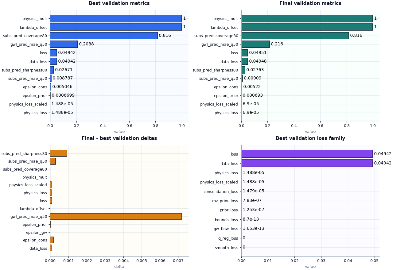
How to interpret these plots#
The first two panels should be read comparatively.
If final validation metrics remain close to best validation metrics, the run probably stayed stable.
If final values become much worse, the run may have drifted after the best checkpoint.
The delta plot makes that easier to see:
values near zero usually mean stability,
large positive deltas for losses or MAE often suggest degradation,
and sharp changes in epsilon metrics may indicate the physics side became less consistent late in training.
The loss-family plot should also be read structurally. In many healthy runs, the main loss is still dominated by data loss, with physics-side terms remaining smaller and controlled. If one auxiliary term suddenly dominates, that is often worth auditing.
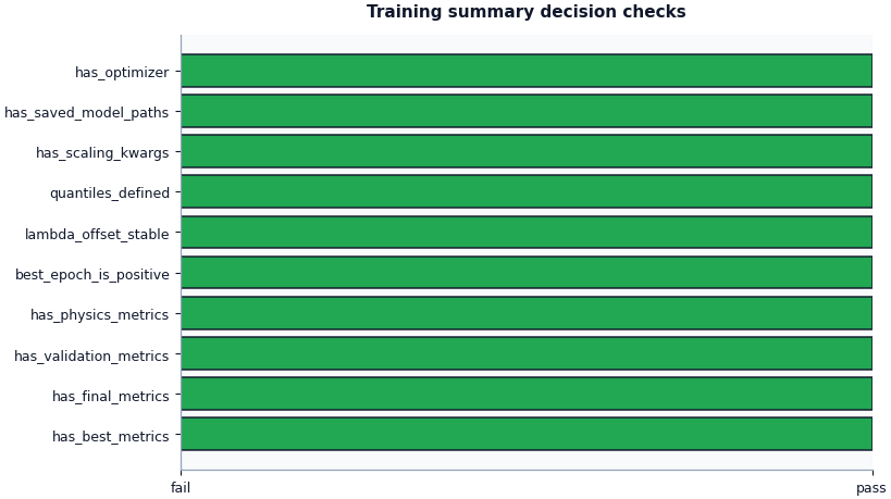
Plot the structural checks separately#
The boolean summary compresses the most important semantic checks into a pass/fail style view.
This is helpful when triaging many runs because it immediately answers whether the summary contains the minimum structural pieces needed for a trustworthy review.
Save a full inspection bundle#
The all-in-one inspector can also write a compact figure bundle. This pattern is useful for later reporting and for gallery pages that want reproducible saved outputs in addition to inline plots.
bundle_dir = out_dir / "inspection_bundle"
bundle_with_figs = inspect_training_summary(
    summary_record,
    output_dir=bundle_dir,
    stem="lesson_training_summary",
    save_figures=True,
)

print("\nSaved inspection figures")
for name, path in bundle_with_figs["figure_paths"].items():
    print(f" - {name}: {path}")
Saved inspection figures
 - lesson_training_summary_best_val_metrics.png: /tmp/gp_training_summary_ce1z2xtr/inspection_bundle/lesson_training_summary_best_val_metrics.png
 - lesson_training_summary_final_val_metrics.png: /tmp/gp_training_summary_ce1z2xtr/inspection_bundle/lesson_training_summary_final_val_metrics.png
 - lesson_training_summary_delta_val_metrics.png: /tmp/gp_training_summary_ce1z2xtr/inspection_bundle/lesson_training_summary_delta_val_metrics.png
 - lesson_training_summary_best_val_losses.png: /tmp/gp_training_summary_ce1z2xtr/inspection_bundle/lesson_training_summary_best_val_losses.png
 - lesson_training_summary_checks.png: /tmp/gp_training_summary_ce1z2xtr/inspection_bundle/lesson_training_summary_checks.png
A practical reading rule#
A simple decision rule for this artifact family can be:
both best and final metrics exist,
validation metrics exist,
physics metrics exist,
a clear optimizer is recorded,
scaling kwargs are preserved,
and the main saved model paths are present.
If those checks pass, then the training summary is usually rich enough to support downstream evaluation decisions.
After that, interpret the run qualitatively:
small best-vs-final drifts usually suggest stable training,
reasonable coverage/sharpness balance suggests usable interval behavior,
and controlled epsilon metrics suggest the physics side did not become pathological.
checks = summary["checks"]
must_pass = [
    "has_best_metrics",
    "has_final_metrics",
    "has_validation_metrics",
    "has_physics_metrics",
    "has_saved_model_paths",
    "has_optimizer",
    "has_scaling_kwargs",
]
ready = all(bool(checks.get(name, False)) for name in must_pass)

print("\nDecision note")
if ready:
    print(
        "This demo training summary looks structurally ready "
        "for deeper evaluation and downstream workflow review."
    )
else:
    print(
        "This training summary needs attention before you rely "
        "on the run downstream."
    )
Decision note
This demo training summary looks structurally ready for deeper evaluation and downstream workflow review.
Total running time of the script: (0 minutes 1.556 seconds)