Inspection

This gallery focuses on workflow-artifact inspection in GeoPrior.

The pages in this section are built as guided lessons for users who already ran part of the workflow and now want to answer a practical question before moving on:

What do the saved artifacts actually say, and are they trustworthy enough to justify the next decision?

That is the central purpose of this gallery.

Unlike the forecasting gallery, which teaches how forecast outputs are built and interpreted, and unlike the diagnostics gallery, which focuses on workflow validity, training curves, and tuning behavior, the pages in this section are organized around a different object:

the saved artifact itself.

These lessons teach users how to read files such as:

• Stage-1 audits,

• Stage-1 manifests,

• resolved scaling_kwargs.json files,

• model-initialization manifests,

• Stage-2 run manifests,

• training summaries,

• calibration stats,

• compact evaluation diagnostics,

• interpretable evaluation-physics payloads,

• physics-payload metadata sidecars,

• transfer-result bundles,

• ablation experiment logs.

In other words, this gallery is about reading workflow evidence. It helps users inspect what the workflow saved, understand what each file means, and decide whether to continue, recalibrate, compare, export, or re-run.

Why this gallery exists

GeoPrior writes many useful artifacts during Stage-1, Stage-2, calibration, evaluation, export, and transfer workflows. Those files are valuable because they preserve:

• what was configured,

• what was actually resolved,

• what dimensions and conventions were used,

• what metrics were achieved,

• which paths were exported,

• and which assumptions were active when the result was saved.

But those files are only helpful if a user can read them confidently. A raw JSON file or JSONL log often answers important workflow questions, but not in a form that is easy to interpret quickly.

This gallery therefore turns artifact inspection into a sequence of lessons. Each page shows how to:

1. generate or load a realistic artifact,

2. convert the important nested sections into tidy tables,

3. plot a few key inspection views,

4. explain what each view means,

5. and end with a practical decision rule.

The goal is not only to display artifacts. The goal is to teach users how to reason from the artifact.

What this gallery teaches

Most lessons in this section follow the same broad structure:

1. introduce the workflow question the artifact helps answer,

2. generate a stable demo artifact or load a real one,

3. inspect the compact semantic summary first,

4. read the most important sections as tables,

5. visualize a few decision-oriented views,

6. explain what looks healthy, suspicious, incomplete, or inconsistent,

7. finish with a concrete go / review / caution rule.

That structure matters. It means the examples are not only API demos. They are meant to function as inspection training pages for users who want to understand their own artifacts later.

What this gallery is not

This section does not aim to:

• build final publication figures,

• replace the deeper model-inspection helpers,

• rerun the whole training workflow,

• or explain every modeling concept from first principles.

Instead, it focuses on one practical job:

teach the user how to inspect saved artifacts before making workflow choices.

A useful rule of thumb is:

• forecasting/ explains forecast outputs and forecast-facing helpers,

• uncertainty/ explains interval calibration and uncertainty reading,

• diagnostics/ explains workflow validity, split credibility, training curves, and tuning behavior,

• model_inspection/ explains deeper internals and learned quantities,

• inspection/ explains how to read the saved artifact files that tie those workflow stages together.

Module guide

Module	Main output	Purpose
plot_stage1_audit_overview.py	Stage-1 audit reading lesson	Inspect coordinate normalization, feature-bucket structure, Stage-1 variable statistics, target summaries, and early preprocessing credibility before looking at downstream artifacts.
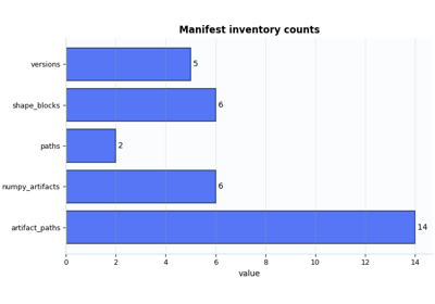
plot_manifest_overview.py	Stage-1 manifest reading lesson	Inspect the broader preprocessing handshake: config snapshot, feature groups, holdout counts, artifact inventory, paths, versions, and shape summaries.
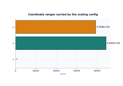
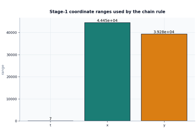
plot_scaling_kwargs_overview.py	Scaling configuration lesson	Read the resolved scaling sidecar that controls SI affine maps, coordinate conventions, groundwater interpretation, forcing semantics, bounds, schedules, and feature-channel identities.
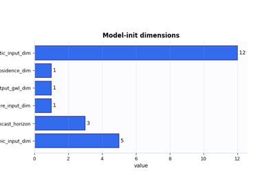
plot_model_init_manifest_overview.py	Model-init manifest lesson	Inspect the initialized model contract before training: dimensions, architecture choices, GeoPrior physics-init knobs, feature-group counts, and the scaling view resolved at init time.
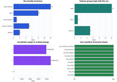
plot_run_manifest_overview.py	Run-manifest lesson	Inspect the lightweight Stage-2 bundle that records run identity, compact config, exported paths, and direct artifact pointers.
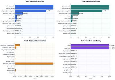
plot_training_summary_overview.py	Training-summary lesson	Compare best versus final metrics, train versus validation behavior, physics-loss balance, uncertainty metrics, and saved outputs before trusting a run downstream.
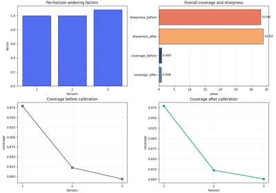
plot_calibration_stats_overview.py	Calibration-stats lesson	Read per-horizon calibration factors and the before/after coverage-sharpness trade-off to decide whether interval calibration actually helped.
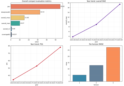
plot_eval_diagnostics_overview.py	Compact evaluation lesson	Inspect overall forecast quality, year-by-year drift, per-horizon degradation, interval behavior, and prediction stability from the compact diagnostics artifact.
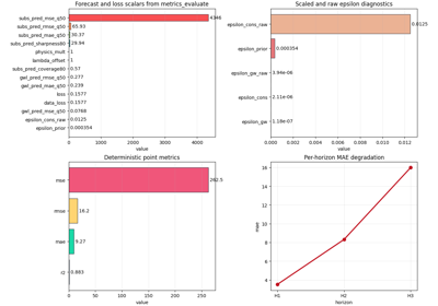
plot_eval_physics_overview.py	Interpretable eval-physics lesson	Read forecast metrics, epsilon diagnostics, calibration blocks, censor-aware summaries, per-horizon behavior, and units together in one evaluation checkpoint.
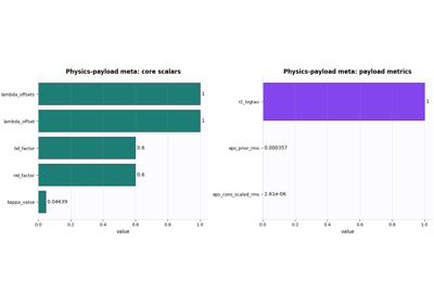
plot_physics_payload_meta_overview.py	Physics payload metadata lesson	Confirm PDE modes, closure assumptions, groundwater conventions, units, and compact payload metrics before opening the heavier NPZ payload.
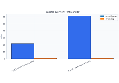
plot_xfer_results_overview.py	Transfer-results lesson	Compare cross-city transfer directions, strategies, calibration/rescaling choices, schema mismatch, warm-start setup, and per-horizon behavior side by side.
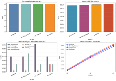
plot_ablation_record_overview.py	Ablation-record lesson	Read the JSONL experiment log as a structured comparison tool for variants, lambda-weight choices, epsilon behavior, and horizon-wise trade-offs rather than as isolated scalar scores.

Suggested reading paths

There is no single correct order, but three reading paths are especially useful.

Stage-1 preparation path

Choose this path when you want to know whether preprocessing outputs are healthy enough for training.

Recommended order:

1. plot_stage1_audit_overview.py

2. plot_manifest_overview.py

3. plot_scaling_kwargs_overview.py

This path helps answer questions such as:

• Were the coordinates normalized the way I expected?

• Which feature groups were actually exported?

• Are the scaling conventions and units ready for Stage-2?

Stage-2 readiness path

Choose this path when the model has been initialized or trained and you want to verify that the run bundle looks structurally trustworthy.

Recommended order:

1. plot_model_init_manifest_overview.py

2. plot_run_manifest_overview.py

3. plot_training_summary_overview.py

This path helps answer questions such as:

• Did the initialized model really use the dimensions and physics knobs I intended?

• Did Stage-2 export the files I expect?

• Does the training summary support trusting the run?

Evaluation and reporting path

Choose this path when the run already finished and you now want to judge forecast quality, calibration quality, and physics-consistency for analysis or reporting.

Recommended order:

1. plot_calibration_stats_overview.py

2. plot_eval_diagnostics_overview.py

3. plot_eval_physics_overview.py

4. plot_physics_payload_meta_overview.py

This path helps answer questions such as:

• Did calibration improve coverage enough to justify the added width?

• Are the compact forecast metrics stable enough to trust?

• Do the interpretable evaluation and metadata support reporting the result confidently?

Comparison and robustness path

Choose this path when the real task is selecting among alternatives.

Recommended order:

1. plot_xfer_results_overview.py

2. plot_ablation_record_overview.py

This path helps answer questions such as:

• Which transfer direction is stronger and why?

• Is schema mismatch driving weak transfer?

• Which ablation setting improves one metric while damaging another?

• Which variant is safest across horizons instead of only best on one scalar metric?

How to use these lessons with real files

Most inspection pages begin by generating a realistic demo artifact. That is useful for documentation because it gives stable examples. However, the real workflow value comes from replacing the demo path with one of your own saved files.

A practical pattern is:

1. run the workflow,

2. locate the saved artifact under results/...,

3. open the matching lesson in this gallery,

4. replace the demo path with your real file,

5. compare the lesson’s reading logic with your own artifact.

This is one of the main goals of the inspection gallery: the examples should remain useful after the user has already run GeoPrior.

How to read the plots in this section

Most plots in this gallery are intentionally simple. They are not final figures for publication. They are decision plots.

That means they are meant to answer questions like:

• Do the counts look complete?

• Do the coordinate ranges look plausible?

• Are the expected feature groups present?

• Did best and final metrics drift too far apart?

• Did calibration improve coverage at an acceptable sharpness cost?

• Is one variant consistently weaker at longer horizons?

When reading these pages, users should usually ask:

What decision does this plot support?

That question keeps the inspection task practical and prevents the user from treating the artifact as passive metadata.

Why artifact inspection matters

In a workflow like GeoPrior, many later mistakes can be traced back to a small earlier mismatch:

• a coordinate convention that changed silently,

• a missing feature group,

• a scaling sidecar with the wrong forcing semantics,

• a run bundle missing one expected file,

• a calibration step that improved coverage but destroyed sharpness,

• a transfer result weakened mainly by schema mismatch,

• an ablation variant that looks good in aggregate but fails at the longest horizon.

Artifact inspection helps catch those issues earlier and more clearly. That is why this gallery is intentionally positioned between:

• workflow execution,

• model evaluation,

• and scientific interpretation.

Notes

• These pages are intentionally lesson-oriented and interpretation-first.

• Most examples use compact synthetic or template-based artifacts so the documentation remains stable and fast to build.

• The goal is not only to show what the helper returns, but to teach how a user should read the result.

• A good practical sequence is:

  • inspect Stage-1 outputs first,

  • inspect Stage-2 init and run manifests next,

  • inspect training, calibration, and evaluation artifacts after that,

  • then move to comparison-oriented artifacts such as transfer results and ablation logs.

Inspect ablation records before choosing a configuration

Inspect ablation records before choosing a configuration

Inspect calibration statistics before trusting interval forecasts

Inspect calibration statistics before trusting interval forecasts

Inspect compact evaluation diagnostics before trusting forecast quality

Inspect compact evaluation diagnostics before trusting forecast quality

Inspect interpretable evaluation physics before reporting results

Inspect interpretable evaluation physics before reporting results

Inspect a Stage-1 manifest before downstream stages

Inspect a Stage-1 manifest before downstream stages

Inspect a model-initialization manifest before training

Inspect a model-initialization manifest before training

Inspect physics-payload metadata before opening the full payload

Inspect physics-payload metadata before opening the full payload

Inspect a Stage-2 run manifest before downstream workflow steps

Inspect a Stage-2 run manifest before downstream workflow steps

Inspect a scaling_kwargs.json configuration

Inspect a scaling_kwargs.json configuration

Inspect a Stage-1 audit before Stage-2

Inspect a Stage-1 audit before Stage-2

Inspect a training summary before trusting a Stage-2 run

Inspect a training summary before trusting a Stage-2 run

Inspect transfer-learning results before trusting cross-city conclusions

Inspect transfer-learning results before trusting cross-city conclusions