
Evaluation#
This gallery focuses on forecast-evaluation plotting in GeoPrior.
The pages in this section are built as guided lessons for users who already have model predictions, forecast tables, interval forecasts, or ensemble outputs and now want to answer a practical question:
How good is this forecast, where does it fail, and which evaluation view should I trust for the next decision?
That is the central purpose of this gallery.
Unlike the forecasting gallery, which focuses on visualizing forecast paths, forecast tables, temporal trajectories, and spatial forecast maps, the pages in this section are organized around a different job:
turning forecasts into interpretable evidence about forecast quality.
These lessons teach users how to read evaluation views such as:
metric change across forecast horizon,
direct forecast comparisons,
radar summaries across segments or score families,
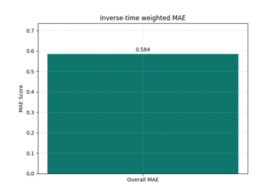
time-weighted summaries that emphasize chosen horizons,
prediction-stability views,
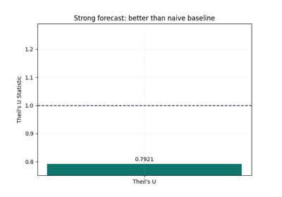
naïve-benchmark skill via Theil’s U,
interval coverage,
interval width and sharpness,
weighted interval score,
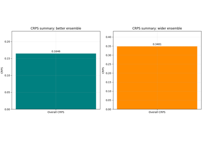
continuous ranked probability score,
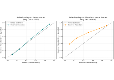
quantile calibration,
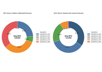
compact QCE summaries,
and final multi-metric score radars.
In other words, this gallery is about judging forecast quality from multiple angles. It helps users decide whether a forecast is accurate, stable, calibrated, sharp enough to be useful, and strong enough to report, compare, or improve.
Why this gallery exists#
A single evaluation number is rarely enough.
A model can look strong on one metric while still being weak in one of several important ways:
short horizons may be strong while long horizons degrade sharply,
interval coverage may improve only because intervals became too wide,
a forecast may be accurate on average but unstable across time,
calibration may look acceptable globally while failing at specific quantiles,
and one model may win on one score while losing on the decision rule that matters most for the task.
This gallery therefore turns evaluation into a sequence of lessons. Each page shows how to:
prepare a small, realistic forecast example,
call one evaluation plotting helper,
explain what the plot is actually measuring,
show what healthy and unhealthy patterns look like,
and finish with a practical rule for using the same logic on real outputs.
The goal is not only to display scores. The goal is to teach users how to reason from the evaluation view.
What this gallery teaches#
Most lessons in this section follow the same broad structure:
introduce the evaluation question the plot helps answer,
build a stable toy example with point, interval, or quantile forecasts,
call the plotting helper in its simplest useful mode,
explain how to read the figure before making a decision,
add a second or third usage pattern,
finish with a checklist for adapting the helper to real forecast arrays or real forecast tables.
That structure matters. It means the examples are not only API demos. They are meant to function as evaluation training pages for users who want to inspect their own forecasts later.
What this gallery is not#
This section does not aim to:
replace the forecasting gallery for raw forecast visualization,
replace the diagnostics gallery for workflow validity or training behavior,
present final publication figures as the main goal,
or reduce forecast quality to a single ranking number.
Instead, it focuses on one practical job:
teach the user which evaluation plot to use, what it means, and what kind of forecast decision it supports.
A useful rule of thumb is:
forecasting/explains what the forecasts look like,evaluation/explains how good those forecasts are,diagnostics/explains whether the workflow and training process behind them look trustworthy,inspection/explains how to read the saved artifacts generated by those workflows.
Module guide#
Module |
Main output |
Purpose |
|---|---|---|
|
Horizon-wise metric lesson |
Learn how point or interval-oriented metrics change across forecast steps, how to compare grouped subsets, and how to spot long-horizon degradation before relying on one global score. |
|
Forecast-comparison lesson |
Compare forecast paths directly in temporal or spatial form so users can connect score summaries back to what the model is actually predicting. |
|
Segment-radar lesson |
Compare one chosen metric across segments, groups, or categories to see where performance concentrates or breaks down. |
|
Time-weighted metric lesson |
Emphasize specific horizons through inverse-time or custom weights and learn when a weighted score tells a more useful story than an unweighted average. |
|
Stability lesson |
Read prediction stability as a complementary quality signal and learn when forecast paths are too erratic even if average error looks acceptable. |
|
Relative-skill lesson |
Benchmark forecasts against a naïve reference using Theil’s U and decide whether the model is truly beating a simple persistence strategy. |
|
Coverage lesson |
Inspect whether interval forecasts cover observations often enough and learn why coverage alone is useful but insufficient. |
|
Width lesson |
Read interval width as a sharpness view and judge whether the forecast is informative or only safe because intervals are broad. |
|
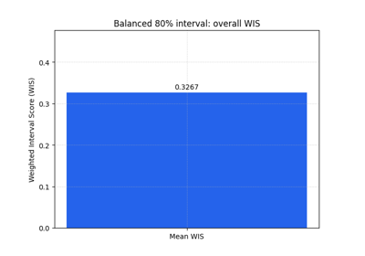
WIS lesson |
Combine interval width and miss penalties into one score and learn how to read the trade-off between sharpness and reliability. |
|
CRPS lesson |
Evaluate full predictive distributions or ensembles with a score that rewards both concentration and correctness. |
|
Quantile-calibration lesson |
Compare nominal and empirical quantile behavior to determine whether quantile forecasts are calibrated across the distribution. |
|
QCE-summary lesson |
Read compact quantile calibration error as an at-a-glance summary of where calibration gaps remain across quantile levels. |
|
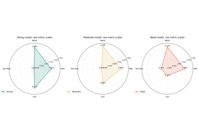
Multi-score radar lesson |
Build compact score profiles across categories or metrics and use them as a final synthesis view for comparison-oriented reporting. |
Suggested reading paths#
There is no single correct order, but four reading paths are especially useful.
Point-forecast quality path#
Choose this path when you first want to know whether the point forecast itself is useful.
Recommended order:
plot_metric_over_horizon_overview.pyplot_forecast_comparison_overview.pyplot_time_weighted_metric_overview.pyplot_theils_u_score_overview.py
This path helps answer questions such as:
Do later horizons become much harder?
Does the forecast path look reasonable when plotted directly?
Should near-term or long-term horizons matter more in my summary?
Is the model really beating a simple baseline?
Uncertainty and interval-quality path#
Choose this path when your forecast includes uncertainty bounds and you want to judge whether those bounds are believable and useful.
Recommended order:
plot_coverage_overview.pyplot_mean_interval_width_overview.pyplot_weighted_interval_score_overview.pyplot_crps_overview.py
This path helps answer questions such as:
Are the intervals covering observations often enough?
Are they too wide to be decision-useful?
Does a better score come from better calibration or just wider bands?
Does the full predictive distribution still look strong when judged as a distribution, not only as a median path?
Calibration-reading path#
Choose this path when your main concern is whether quantiles and probabilities are aligned with observed frequencies.
Recommended order:
plot_quantile_calibration_overview.pyplot_qce_donut_overview.py
This path helps answer questions such as:
Which quantiles are over- or under-covering?
Is the calibration error concentrated in the tails or spread across all quantiles?
Does the forecast need recalibration before reporting?
Comparison and synthesis path#
Choose this path when you need a compact comparison across segments, outputs, or score families.
Recommended order:
plot_metric_radar_overview.pyplot_prediction_stability_overview.pyplot_radar_scores_overview.py
This path helps answer questions such as:
Which segment or subgroup is hardest?
Is one model smoother but less accurate?
Which score profile best matches the decision rule that matters for my application?
How to use these lessons with real forecast outputs#
Most evaluation pages begin with small synthetic or hand-built forecast examples. That is useful for documentation because it keeps the lesson stable and easy to read.
However, the real workflow value comes from replacing those demo arrays or demo tables with your own outputs.
A practical pattern is:
export or collect the forecast outputs you want to evaluate,
identify whether you have point forecasts, interval forecasts, quantile tables, or ensembles,
open the matching lesson in this gallery,
replace the demo arrays or DataFrame with your real outputs,
check that column names and shapes follow the helper’s expected contract,
and then read the plot using the same interpretation logic taught on the page.
This is one of the main goals of the evaluation gallery: the examples should remain useful after the user already has real forecast results.
How to read the plots in this section#
Most plots in this gallery are intentionally practical. They are not only decorative figures. They are decision plots.
That means they are meant to answer questions like:
Where does error rise across the forecast horizon?
Is the model better than a naïve baseline?
Are intervals calibrated or merely wide?
Does one output behave differently from the others?
Which quantiles are failing calibration?
Which metric profile best fits the reporting goal?
When reading these pages, users should usually ask:
What forecast decision does this plot support?
That question keeps evaluation practical and prevents the user from reducing forecast quality to a single number too early.
Why multi-view evaluation matters#
In a forecasting workflow like GeoPrior, weak decisions often come from looking at one score in isolation:
low MAE may hide poor long-horizon behavior,
acceptable coverage may hide intervals that are too wide,
good calibration at one quantile may hide tail failures,
a strong score average may hide one unstable output,
and a smooth forecast may still underperform a naïve baseline.
Multi-view evaluation helps catch those cases earlier and more clearly. That is why this gallery is intentionally positioned between:
forecast generation,
calibration and evaluation reading,
and model comparison or reporting.
Notes#
These pages are intentionally lesson-oriented and interpretation-first.
Most examples use compact synthetic or template-like forecast arrays so the documentation remains stable and quick to build.
The goal is not only to show what a plotting helper returns, but to teach how a user should read the result.
A good practical sequence is:
start with horizon-wise error and direct forecast comparison,
then inspect interval quality and probabilistic scores,
then inspect quantile calibration,
and finally use radar-style summaries for compact comparison.
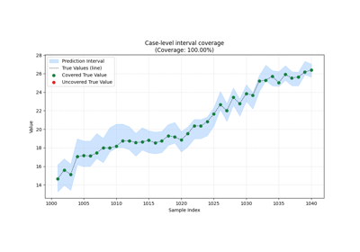
Learn how to read interval reliability with plot_coverage
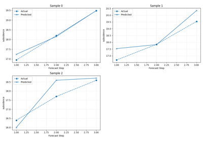
Learn to compare forecasts visually with plot_forecast_comparison
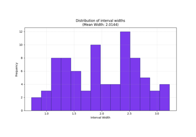
Learn how to read forecast sharpness with plot_mean_interval_width
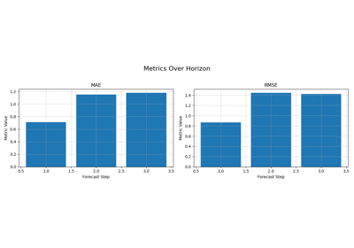
Read forecast quality horizon by horizon with plot_metric_over_horizon
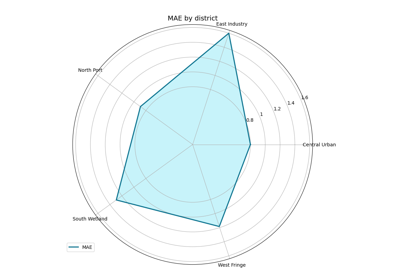
Compare forecast quality across groups with plot_metric_radar
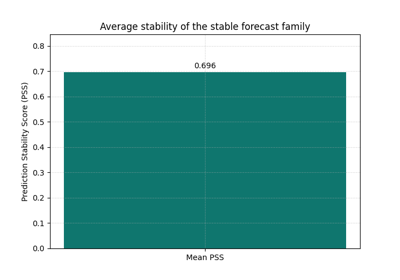
Learn how forecast smoothness behaves with plot_prediction_stability
Read quantile reliability with plot_quantile_calibration
Compare compact score profiles with plot_radar_scores
Learn how to benchmark a forecast against a naive baseline with plot_theils_u_score
Learn how horizon emphasis changes the score with plot_time_weighted_metric
Learn how to judge interval forecasts with plot_weighted_interval_score