
Note
Go to the end to download the full example code.
Extract threshold-based spatial zones with extract-zones#
This lesson teaches how to build compact zone tables from a spatial
field using GeoPrior’s extract-zones workflow.
Unlike ROI extraction, which cuts out one rectangular window, this builder keeps only the points whose target value satisfies a threshold rule. That makes it a natural tool for:
hotspot extraction,
low-score or vulnerable-zone screening,
transition-band inspection,
and small zone tables that can be passed to later summaries or plots.
Why this matters#
Threshold-based extraction is one of the simplest and most practical ways to turn a continuous spatial score into a reusable table of points.
In many applied workflows, the first useful question is not:
“What does the full field look like?”
It is:
“Which points are above a critical level?”
or
“Which points fall in the lower-risk tail?”
That is the role of extract-zones.
What this lesson teaches#
We will:
build a realistic synthetic spatial table,
save it as two separate input files,
extract three different zone types,
compare their thresholds and sizes,
build one compact visual preview,
end with direct command-line examples.
Imports#
We use the real zone-extraction helper from GeoPrior and the shared synthetic spatial helpers already used in the other gallery lessons.
from __future__ import annotations

import tempfile
from pathlib import Path

import matplotlib.pyplot as plt
import numpy as np
import pandas as pd

from geoprior.utils.spatial_utils import extract_zones_from
from geoprior.scripts import utils as script_utils
Step 1 - Build one reusable synthetic city support#
Instead of generating plain random coordinates, we reuse the shared support helper. That gives us a more city-like footprint and keeps the lesson visually consistent with the other build examples.
Key parameters#
- city:
Only a label attached to the synthetic support.
- center_x, center_y:
Center of the projected coordinate system.
- span_x, span_y:
Half-width and half-height of the support extent.
- nx, ny:
Mesh density before masking.
- jitter_x, jitter_y:
Small perturbations so the support is not a perfect mesh.
- footprint:
Shape of the retained support.
- keep_frac:
Fraction of masked points to keep.
- seed:
Reproducibility seed.
support = script_utils.make_spatial_support(
    script_utils.SpatialSupportSpec(
        city="ZonesDemo",
        center_x=5_000.0,
        center_y=3_100.0,
        span_x=4_800.0,
        span_y=3_400.0,
        nx=35,
        ny=27,
        jitter_x=30.0,
        jitter_y=24.0,
        footprint="nansha_like",
        keep_frac=0.92,
        seed=303,
    )
)
Step 2 - Turn the support into a synthetic spatial score table#
extract_zones_from works on one score variable z and optional
coordinate variables x and y. To make the lesson realistic, we
build one continuous score field that looks like an interpretable urban
response surface.
The score can be read as a generic hazard, severity, or hotspot index. The exact semantics are not important here. The important point is that it is continuous, spatially structured, and suitable for thresholding.
rng = np.random.default_rng(303)

base_field = script_utils.make_spatial_field(
    support,
    amplitude=2.45,
    drift_x=1.10,
    drift_y=0.35,
    phase=0.50,
    local_weight=0.18,
)

spread_field = script_utils.make_spatial_scale(
    support,
    base=0.25,
    x_weight=0.10,
    hotspot_weight=0.07,
)

city_df = support.to_frame().copy()
city_df["district"] = np.where(
    city_df["x_norm"] > 0.62,
    "East corridor",
    np.where(city_df["y_norm"] > 0.58, "North belt", "Urban core"),
)
city_df["susceptibility_score"] = (
    6.2
    + 1.85 * base_field
    + 1.10 * spread_field
    + rng.normal(0.0, 0.18, len(city_df))
)
city_df["rainfall_mm"] = (
    1180
    + 95 * city_df["y_norm"]
    + rng.normal(0.0, 10.0, len(city_df))
)
city_df["groundwater_depth_m"] = (
    8.4
    + 0.9 * city_df["x_norm"]
    + 0.5 * city_df["y_norm"]
    + rng.normal(0.0, 0.08, len(city_df))
)

print("Synthetic table shape:", city_df.shape)
print("")
print(city_df.head(10).to_string(index=False))
Synthetic table shape: (414, 10)

 sample_idx   coord_x  coord_y  x_norm  y_norm      city      district  susceptibility_score  rainfall_mm  groundwater_depth_m
          0 3654.7573 725.7191  0.3621  0.1582 ZonesDemo    Urban core                7.8543    1196.5087               8.8016
          1 3879.0054 716.6930  0.3851  0.1569 ZonesDemo    Urban core                7.8991    1203.0117               8.8067
          2 4127.1475 743.3290  0.4106  0.1608 ZonesDemo    Urban core                7.8215    1196.6609               8.9188
          3 4530.8041 743.3618  0.4521  0.1608 ZonesDemo    Urban core                8.0307    1166.7556               8.7492
          4 4741.9471 747.9166  0.4737  0.1615 ZonesDemo    Urban core                7.8903    1208.5079               9.0510
          5 4987.8599 751.7753  0.4990  0.1620 ZonesDemo    Urban core                8.3513    1191.2383               8.8633
          6 5290.1053 760.6047  0.5300  0.1633 ZonesDemo    Urban core                7.9618    1193.3879               9.1051
          7 5554.3981 728.7704  0.5572  0.1587 ZonesDemo    Urban core                8.0325    1199.9865               9.0134
          8 5886.9462 751.2118  0.5913  0.1619 ZonesDemo    Urban core                8.1350    1184.2525               8.9630
          9 6363.0598 730.2099  0.6402  0.1589 ZonesDemo East corridor                8.5844    1211.7271               9.0817
Step 3 - Save the table as two input files#
The public build layer accepts one or many input tables. To make that visible in the lesson, we split the synthetic city into two files and conceptually rebuild the same combined table again.
tmp_dir = Path(
    tempfile.mkdtemp(prefix="gp_sg_extract_zones_")
)

west_csv = tmp_dir / "zones_demo_west.csv"
east_csv = tmp_dir / "zones_demo_east.csv"

x_mid = float(city_df["coord_x"].median())
city_df.loc[city_df["coord_x"] <= x_mid].to_csv(
    west_csv,
    index=False,
)
city_df.loc[city_df["coord_x"] > x_mid].to_csv(
    east_csv,
    index=False,
)

print("")
print("Input files")
print(" -", west_csv.name)
print(" -", east_csv.name)
Input files
 - zones_demo_west.csv
 - zones_demo_east.csv
Step 4 - Define three thresholding stories#
We extract three different kinds of zones from the same score field. This makes the lesson more useful than a single one-off threshold.
low_autolower-tail automatic thresholding using a percentile.hotspotpoints above an explicit upper threshold.transitionpoints inside an intermediate score band.
The explicit thresholds are derived from quantiles so the lesson stays stable even if the synthetic field is adjusted later.
z = city_df["susceptibility_score"].to_numpy(float)
auto_percentile = 15
auto_threshold = float(np.percentile(z, auto_percentile))
hotspot_threshold = float(np.percentile(z, 82))
transition_band = (
    float(np.percentile(z, 46)),
    float(np.percentile(z, 64)),
)

print("")
print("Threshold design")
print(f" - auto lower threshold (p{auto_percentile}) = {auto_threshold:.3f}")
print(f" - hotspot threshold = {hotspot_threshold:.3f}")
print(
    " - transition band = "
    f"({transition_band[0]:.3f}, {transition_band[1]:.3f})"
)
Threshold design
 - auto lower threshold (p15) = 8.080
 - hotspot threshold = 10.528
 - transition band = (8.865, 9.539)
Step 5 - Extract the three zone tables#
We call the real extraction helper directly. The public CLI command is a thin convenience layer over the same threshold logic.
extract_zones_from returns only the filtered coordinate and score
columns, which is exactly what we want for compact zone exports.
def _zone_table(
    data: pd.DataFrame,
    *,
    threshold,
    condition: str,
    percentile: int | float = 10,
    use_negative_criteria: bool = True,
) -> pd.DataFrame:
    out = extract_zones_from(
        z="susceptibility_score",
        x="coord_x",
        y="coord_y",
        data=data,
        threshold=threshold,
        condition=condition,
        use_negative_criteria=use_negative_criteria,
        percentile=percentile,
        view=False,
    )
    out = out.copy()
    out.columns = ["coord_x", "coord_y", "susceptibility_score"]
    return out


low_auto = _zone_table(
    city_df,
    threshold="auto",
    condition="auto",
    percentile=auto_percentile,
    use_negative_criteria=True,
)

hotspot = _zone_table(
    city_df,
    threshold=hotspot_threshold,
    condition="above",
    use_negative_criteria=False,
)

transition = _zone_table(
    city_df,
    threshold=transition_band,
    condition="between",
    use_negative_criteria=False,
)

low_csv = tmp_dir / "zones_demo_low_auto.csv"
hotspot_csv = tmp_dir / "zones_demo_hotspot.csv"
transition_csv = tmp_dir / "zones_demo_transition.csv"

low_auto.to_csv(low_csv, index=False)
hotspot.to_csv(hotspot_csv, index=False)
transition.to_csv(transition_csv, index=False)

print("")
print("Written files")
print(" -", low_csv.name)
print(" -", hotspot_csv.name)
print(" -", transition_csv.name)

print("")
print("Low-score auto zone")
print(low_auto.head(8).to_string(index=False))

print("")
print("Hotspot zone")
print(hotspot.head(8).to_string(index=False))

print("")
print("Transition band")
print(transition.head(8).to_string(index=False))
Written files
 - zones_demo_low_auto.csv
 - zones_demo_hotspot.csv
 - zones_demo_transition.csv

Low-score auto zone
  coord_x   coord_y  susceptibility_score
3654.7573  725.7191                7.8543
3879.0054  716.6930                7.8991
4127.1475  743.3290                7.8215
4530.8041  743.3618                8.0307
4741.9471  747.9166                7.8903
5290.1053  760.6047                7.9618
5554.3981  728.7704                8.0325
2735.5954 1017.2204                7.8516

Hotspot zone
  coord_x   coord_y  susceptibility_score
5902.7448 1802.0862               11.1294
6135.7027 1827.0407               11.6021
6410.7167 1787.5672               11.4881
6684.9167 1765.4587               11.1619
6992.9990 1793.7800               11.4905
7333.2870 1788.1407               10.5601
5313.0400 2046.3373               10.6809
5624.3402 2059.1097               11.0479

Transition band
  coord_x   coord_y  susceptibility_score
6143.2959  980.3361                9.0711
6669.7483 1010.8933                9.0629
6911.9625 1018.0694                9.4021
7317.7457 1030.8998                8.8854
5362.6798 1274.7406                9.1439
6144.5651 1263.2123                9.3788
6678.2034 1285.9056                9.3800
6943.2837 1250.0980                9.2733
Step 6 - Summarize the three outputs#
A small summary table makes it easy to compare how the different threshold rules behave.
def summarize_zone(
    df: pd.DataFrame,
    *,
    label: str,
    threshold_text: str,
) -> dict[str, object]:
    return {
        "zone": label,
        "threshold_rule": threshold_text,
        "rows": int(len(df)),
        "score_min": float(df["susceptibility_score"].min()),
        "score_mean": float(df["susceptibility_score"].mean()),
        "score_max": float(df["susceptibility_score"].max()),
    }


summary = pd.DataFrame(
    [
        summarize_zone(
            low_auto,
            label="low_auto",
            threshold_text=f"auto below p{auto_percentile}",
        ),
        summarize_zone(
            hotspot,
            label="hotspot",
            threshold_text=f"> {hotspot_threshold:.2f}",
        ),
        summarize_zone(
            transition,
            label="transition",
            threshold_text=(
                f"between {transition_band[0]:.2f} and "
                f"{transition_band[1]:.2f}"
            ),
        ),
    ]
)

print("")
print("Zone summary")
print(summary.to_string(index=False))
Zone summary
      zone        threshold_rule  rows  score_min  score_mean  score_max
  low_auto        auto below p15    62     6.7745      7.6908     8.0779
   hotspot               > 10.53    75    10.5367     11.6053    13.4455
transition between 8.87 and 9.54    75     8.8652      9.1966     9.5345
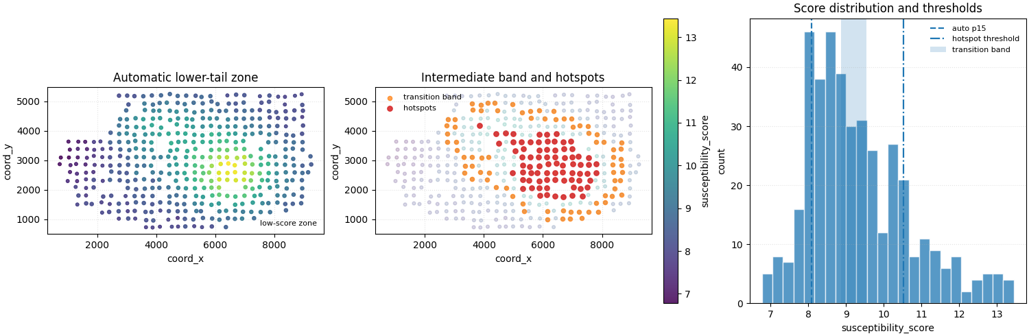
Step 7 - Build one compact visual preview#
- Left:
full score field with the low-score zone overlaid.
- Middle:
full score field with hotspot and transition points overlaid.
- Right:
score histogram with the three threshold rules annotated.
fig, axes = plt.subplots(
    1,
    3,
    figsize=(15.0, 4.9),
    constrained_layout=True,
)

# Panel 1 - lower-tail zone.
ax = axes[0]
sc = ax.scatter(
    city_df["coord_x"],
    city_df["coord_y"],
    c=city_df["susceptibility_score"],
    s=14,
    cmap="viridis",
    alpha=0.86,
)
ax.scatter(
    low_auto["coord_x"],
    low_auto["coord_y"],
    s=32,
    facecolors="none",
    edgecolors="white",
    linewidths=1.2,
    label="low-score zone",
)
ax.set_title("Automatic lower-tail zone")
ax.set_xlabel("coord_x")
ax.set_ylabel("coord_y")
ax.legend(frameon=False, fontsize=8)
ax.grid(True, linestyle=":", alpha=0.35)
ax.set_aspect("equal", adjustable="box")

# Panel 2 - hotspot and transition zones.
ax = axes[1]
ax.scatter(
    city_df["coord_x"],
    city_df["coord_y"],
    c=city_df["susceptibility_score"],
    s=12,
    cmap="viridis",
    alpha=0.20,
)
ax.scatter(
    transition["coord_x"],
    transition["coord_y"],
    s=20,
    color="tab:orange",
    alpha=0.72,
    label="transition band",
)
ax.scatter(
    hotspot["coord_x"],
    hotspot["coord_y"],
    s=28,
    color="tab:red",
    alpha=0.88,
    label="hotspots",
)
ax.set_title("Intermediate band and hotspots")
ax.set_xlabel("coord_x")
ax.set_ylabel("coord_y")
ax.legend(frameon=False, fontsize=8)
ax.grid(True, linestyle=":", alpha=0.35)
ax.set_aspect("equal", adjustable="box")

# Panel 3 - score histogram and thresholds.
ax = axes[2]
ax.hist(
    city_df["susceptibility_score"],
    bins=24,
    alpha=0.75,
    edgecolor="white",
)
ax.axvline(
    auto_threshold,
    linestyle="--",
    linewidth=1.6,
    label=f"auto p{auto_percentile}",
)
ax.axvline(
    hotspot_threshold,
    linestyle="-.",
    linewidth=1.6,
    label="hotspot threshold",
)
ax.axvspan(
    transition_band[0],
    transition_band[1],
    alpha=0.20,
    label="transition band",
)
ax.set_title("Score distribution and thresholds")
ax.set_xlabel("susceptibility_score")
ax.set_ylabel("count")
ax.legend(frameon=False, fontsize=8)
ax.grid(True, axis="y", linestyle=":", alpha=0.35)

# Add one shared colorbar for the spatial panels.
cbar = fig.colorbar(sc, ax=axes[:2], fraction=0.035, pad=0.02)
cbar.set_label("susceptibility_score")

plt.show()
How to read this output#
A useful reading order is:
inspect the continuous score field,
check which threshold rule was applied,
compare the selected point counts,
then compare the score ranges in the exported tables.
The key idea is that the builder is not estimating a new field. It is simply turning one existing continuous score into one reusable point table based on a threshold criterion.
Why this builder is useful in practice#
extract-zones is a strong support-layer builder when you need one
threshold-defined subset rather than a full-city table.
Typical uses include:
extracting hotspot candidates,
isolating the lower-risk or lower-response tail,
creating intermediate bands for sensitivity checks,
or preparing compact point tables for later reports.
Command-line usage#
The examples below show the same workflow as direct terminal commands.
Explicit hotspot extraction#
geoprior-build extract-zones \
    zones_demo_west.csv zones_demo_east.csv \
    --x-col coord_x \
    --y-col coord_y \
    --z-col susceptibility_score \
    --threshold 8.43 \
    --condition above \
    --output zones_demo_hotspot.csv
The same command through the root dispatcher#
geoprior build extract-zones \
    zones_demo_west.csv zones_demo_east.csv \
    --x-col coord_x \
    --y-col coord_y \
    --z-col susceptibility_score \
    --threshold 8.43 \
    --condition above \
    --output zones_demo_hotspot.csv
Intermediate transition band#
geoprior-build extract-zones \
    zones_demo_west.csv zones_demo_east.csv \
    --x-col coord_x \
    --y-col coord_y \
    --z-col susceptibility_score \
    --threshold 6.45 7.28 \
    --condition between \
    --output zones_demo_transition.csv
Lower-tail automatic extraction#
The underlying helper also supports percentile-driven automatic thresholds. When your local wrapper exposes the same options, a typical command looks like:
geoprior-build extract-zones \
    zones_demo_west.csv zones_demo_east.csv \
    --x-col coord_x \
    --y-col coord_y \
    --z-col susceptibility_score \
    --threshold auto \
    --percentile 15 \
    --condition auto \
    --output zones_demo_low_auto.csv
Because the shared reader accepts one or many input tables, the same command family can also be used with CSV, TSV, Parquet, Excel, JSON, Feather, or Pickle inputs.
Total running time of the script: (0 minutes 0.526 seconds)