Tables and summaries#
This gallery focuses on artifact-building workflows in GeoPrior.
Unlike the examples in figure_generation/, the pages collected here
usually do not begin from a final paper figure. They begin from forecast
CSVs, experiment records, Stage-1 artifacts, hotspot point clouds,
processed city tables, and compact synthetic spatial supports, then show
how to turn those materials into clean, reusable outputs.
The emphasis is therefore on builders, not on presentation. These lessons explain how GeoPrior produces the tables, merged datasets, selection subsets, and lightweight spatial layers that later diagnostics, applications, maps, and publication figures depend on.
What this gallery produces#
Typical outputs in this section include:
run-level metric tables,
grouped ablation summaries,
exceedance-scoring tables,
extended or merged forecast artifacts,
forecast-ready demo panels,
manifest-driven NPZ bundles,
spatial samples and non-overlapping batches,
rectangular ROI extracts and threshold-based zones,
cluster-labeled support tables,
nearest-city borehole assignments,
coordinate-enriched datasets with
z_surfand optional head,boundary, grid, exposure, and zone-aware support layers.
In other words, this gallery is about building the intermediate artifacts that make later reporting, debugging, mapping, and interpretation possible.
How these lessons are structured#
Most pages in this section follow the same general pattern:
create or load a compact synthetic input,
call the real GeoPrior builder,
inspect the generated artifact,
add a small preview plot only when it helps explain the result,
finish with the matching command-line usage.
Even when a page contains a map, chart, or spatial preview, the main teaching goal remains the same: to explain the table or reusable artifact produced by the command.
For the newer spatial build lessons, the synthetic inputs often come from the reusable spatial-support utilities rather than from ad hoc random coordinates. That keeps the examples compact while still showing realistic spatial footprints and stable command behavior.
Module guide#
Module |
Main output |
Purpose |
|---|---|---|
|
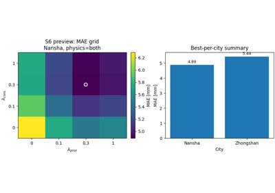
CSV / JSON / TXT / TeX summary tables |
Build tidy ablation archives from sensitivity records, including optional grouped summaries and best-per-city views. |
|
Unified metrics tables |
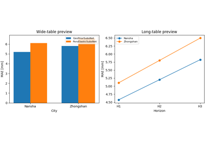
Build wide run-level and long horizon-level metrics tables from experiment outputs. |
|
Exceedance-scoring tables |
Score exceedance events from calibrated forecast quantiles and export tidy Brier-score tables by threshold and year. |
|
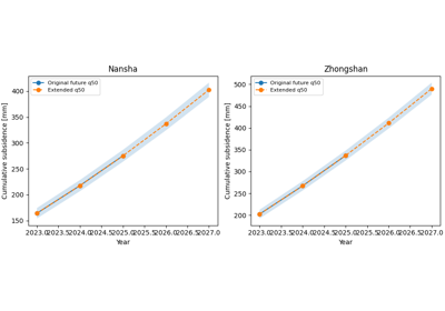
Extended forecast CSVs |
Extend future forecast products to later years using simple extrapolation rules. |
|
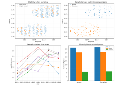
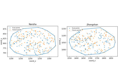
Compact forecast-ready panel sample |
Sample spatial groups rather than rows so the retained subset still preserves enough temporal structure for forecasting demos, tests, and tutorials. |
|
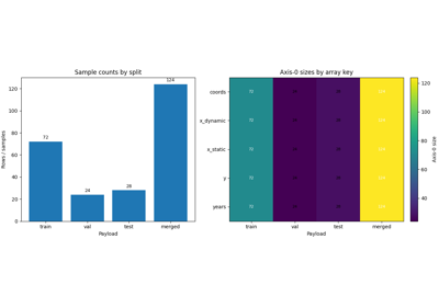
Merged |
Merge split Stage-1 input NPZ artifacts through the manifest into one reusable bundle. |
|
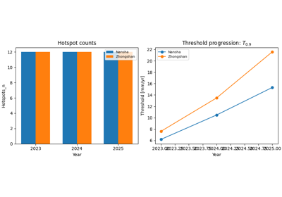
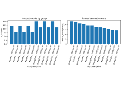
Hotspot summary products |
Build per-city, per-year hotspot summaries relative to a chosen baseline year. |
|
Grouped hotspot tables |
Summarize hotspot point clouds into compact city/year/kind tables for inspection and reuse. |
|
Stratified spatial sample table |
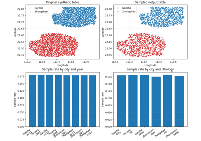
Build one representative sample from one or many input tables by combining spatial bins with optional extra stratification columns. |
|
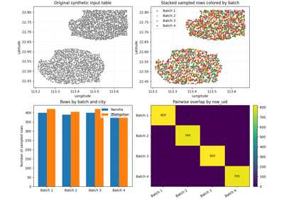
Non-overlapping sampled batches |
Build repeated spatial samples for benchmarking, demos, or batch experiments without reusing the same rows across batches. |
|
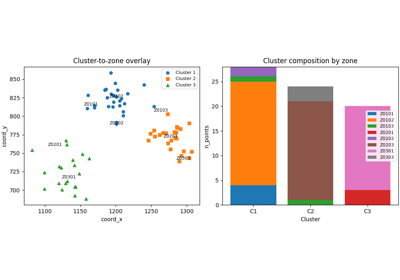
Cluster-labeled spatial table |
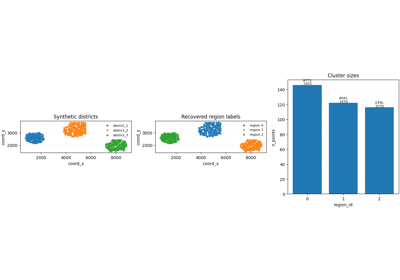
Attach spatial cluster labels to support points using methods such as k-means, DBSCAN, or agglomerative clustering. |
|
Region-of-interest subset table |
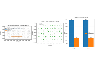
Extract a rectangular spatial window from one or many tabular inputs, with optional snapping to the nearest available support coordinates. |
|
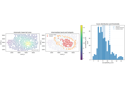
Threshold-based zone table |
Extract high, low, or bounded-response zones from a spatial table using percentile or explicit threshold rules. |
|
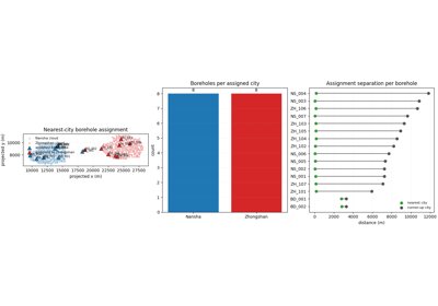
Classified borehole tables |
Assign boreholes to the nearest city support cloud and export one combined table plus optional per-city splits. |
|
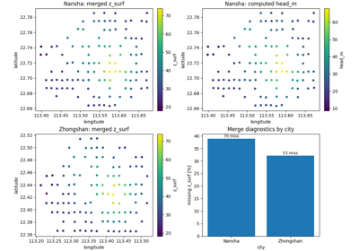
|
Merge rounded coordinate-elevation lookups into city datasets and optionally compute hydraulic head. |
|
Boundary polygons |
Build simple city boundary layers from forecast point clouds. |
|
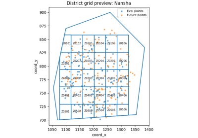
Grid / zone layers |
Build district-style grids over the forecast support domain, optionally clipped to a boundary and linked to samples. |
|
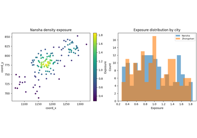
Exposure layer |
Build compact exposure products from sample geometry using uniform or density-based weighting schemes. |
|
Zone-tagged cluster artifacts |
Attach zone identifiers to cluster outputs so they can be interpreted and summarized in a zone-aware way. |
Reading path#
A useful way to move through this gallery is to follow the logic of a real workflow:
start from experiment logs, evaluation records, Stage-1 artifacts, or forecast exports,
turn them into tidy summary tables or merged reusable bundles,
derive compact forecast-ready subsets or extended forecast products,
build spatial samples, batches, ROI selections, zones, or clusters for downstream analysis,
enrich those products with support metadata such as borehole assignment or surface elevation,
continue into diagnostics, hotspot analysis, applications, or figure generation.
That is why the examples are naturally grouped into four broad themes: metric builders, forecast-derived products, spatial sampling and selection tools, and spatial support/enrichment layers.
Gallery organization#
Metrics and experiment summaries#
These examples start from evaluation records, ablation logs, or sensitivity runs and convert them into compact tabular outputs that are much easier to compare, archive, filter, and report.
The main pages in this group are:
build_ablation_table.pybuild_model_metrics.pycompute_brier_exceedance.py
Forecast-derived products and merged inputs#
These examples start from forecast products or Stage-1 split artifacts and build secondary outputs that are easier to inspect, reuse, or carry into later workflow stages.
The main pages in this group are:
extend_forecast.pybuild_forecast_ready_sample.pybuild_full_inputs_npz.pycompute_hotspots.pysummarize_hotspots.py
Spatial sampling and selection tools#
These examples focus on choosing which part of a large spatial table should be kept, grouped, or highlighted before later modelling, inspection, or mapping.
The main pages in this group are:
build_spatial_sampling.pybuild_batch_spatial_sampling.pybuild_spatial_clusters.pybuild_spatial_roi.pybuild_extract_zones.py
Spatial support and enrichment layers#
These examples build or enrich lightweight spatial artifacts that help later analysis stay geographically interpretable.
The main pages in this group are:
build_assign_boreholes.pybuild_add_zsurf_from_coords.pymake_boundary.pymake_district_grid.pymake_exposure.pytag_clusters_with_zones.py
Why this separation matters#
This gallery deliberately keeps four concerns distinct:
data production and merging,
tabulation and forecast-derived summaries,
spatial selection and reduction,
support-layer enrichment and interpretation.
That separation makes the workflow easier to reason about. It also helps users understand which commands generate reusable data products, which commands reduce large tables into compact subsets, which commands add geographic meaning, and which later pages merely visualize the results.
Notes#
These examples are intentionally compact and lesson-oriented.
Many pages include a small preview figure, but that figure is only there to make the artifact easier to understand.
The main output of this gallery is usually a CSV, JSON, TXT, TeX, NPZ, or lightweight spatial layer, not a final publication figure.
Several lessons end with both
geoprior-build ...andgeoprior build ...forms so the reader can move easily between the family-specific entrypoint and the root dispatcher.
Extract threshold-based spatial zones with extract-zones
Build one merged full_inputs.npz from Stage-1 split artifacts
Build unified model-metrics tables from GeoPrior runs
Build spatial cluster tables with spatial-clusters
Extract a rectangular region of interest with spatial-roi
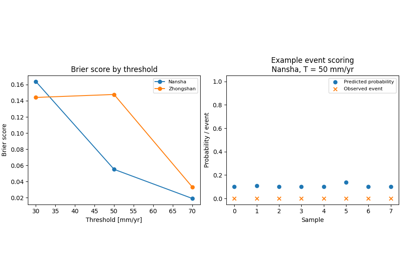
Compute exceedance Brier scores from calibrated forecasts
Create exposure weights from forecast point density
Summarize hotspot point clouds into tidy group tables