
Note
Go to the end to download the full example code.
Build unified model-metrics tables from GeoPrior runs#
This example teaches you how to use GeoPrior’s
build-model-metrics utility.
Unlike the figure-generation scripts, this command is mainly an artifact builder. It scans ablation-record JSONL files across a results tree and turns them into a single unified metrics archive.
Why this matters#
Once you have many runs, you usually need two views:
a wide run-level table for ranking and filtering runs,
a long horizon-level table for forecast-step diagnostics.
This builder produces both from the same source records.
Imports#
We call the production builder, then read its outputs back in and create one compact teaching preview.
from __future__ import annotations

import json
import tempfile
from pathlib import Path

import matplotlib.pyplot as plt
import numpy as np
import pandas as pd

from geoprior.scripts.build_model_metrics import (
    build_model_metrics_main,
)
Build a compact synthetic results tree#
The real builder scans a results root for files like:
<run_dir>/ablation_records/ablation_record*.jsonl
For the lesson, we create a small synthetic results tree with:
two cities,
two model families,
per-horizon MAE and R2,
post-hoc interval-calibration metrics,
and one duplicate run stored both as a legacy record and as an updated record.
That lets the page demonstrate three important behaviors:
recursive discovery,
updated-record preference,
long-table generation.
def _interval_block(
    *,
    cov_uncal: float,
    cov_cal: float,
    shp_uncal: float,
    shp_cal: float,
) -> dict[str, object]:
    """Return a compact interval-calibration payload."""
    return {
        "target": 0.80,
        "coverage80_uncalibrated": float(cov_uncal),
        "coverage80_calibrated": float(cov_cal),
        "sharpness80_uncalibrated": float(shp_uncal),
        "sharpness80_calibrated": float(shp_cal),
        "coverage80_uncalibrated_phys": float(
            max(0.0, cov_uncal - 0.01)
        ),
        "coverage80_calibrated_phys": float(
            max(0.0, cov_cal - 0.01)
        ),
        "sharpness80_uncalibrated_phys": float(
            shp_uncal * 1.03
        ),
        "sharpness80_calibrated_phys": float(
            shp_cal * 1.02
        ),
        "factors_per_horizon": {
            "H1": 1.00,
            "H2": 0.96,
            "H3": 0.92,
        },
        "factors_per_horizon_from_cal_stats": {
            "eval_before": {
                "per_horizon": {
                    "H1": {
                        "coverage": float(cov_uncal - 0.01),
                        "sharpness": float(shp_uncal * 0.95),
                    },
                    "H2": {
                        "coverage": float(cov_uncal),
                        "sharpness": float(shp_uncal),
                    },
                    "H3": {
                        "coverage": float(cov_uncal + 0.01),
                        "sharpness": float(shp_uncal * 1.06),
                    },
                }
            },
            "eval_after": {
                "per_horizon": {
                    "H1": {
                        "coverage": float(cov_cal - 0.01),
                        "sharpness": float(shp_cal * 0.95),
                    },
                    "H2": {
                        "coverage": float(cov_cal),
                        "sharpness": float(shp_cal),
                    },
                    "H3": {
                        "coverage": float(cov_cal + 0.01),
                        "sharpness": float(shp_cal * 1.06),
                    },
                }
            },
        },
    }


def _make_record(
    *,
    timestamp: str,
    city: str,
    model: str,
    pde_mode: str,
    mae_mm: float,
    r2: float,
    lambda_prior: float,
    lambda_cons: float,
    legacy_meters: bool = False,
    add_interval: bool = True,
) -> dict[str, object]:
    """Create one synthetic ablation-style record."""
    rmse_mm = mae_mm * 1.17
    mse_mm2 = rmse_mm**2

    coverage80 = float(
        np.clip(0.90 - 0.01 * (mae_mm - 5.0), 0.72, 0.96)
    )
    sharpness80 = 12.5 + 0.8 * mae_mm

    rec: dict[str, object] = {
        "timestamp": timestamp,
        "city": city,
        "model": model,
        "pde_mode": pde_mode,
        "use_effective_h": bool(city == "Zhongshan"),
        "kappa_mode": "bar" if city == "Nansha" else "kb",
        "hd_factor": 0.6 if city == "Zhongshan" else 1.0,
        "lambda_cons": float(lambda_cons),
        "lambda_gw": 0.2 if pde_mode == "both" else 0.0,
        "lambda_prior": float(lambda_prior),
        "lambda_smooth": 0.3 if lambda_prior >= 0.2 else 0.0,
        "lambda_mv": 0.06 if lambda_cons >= 0.1 else 0.0,
        "r2": float(r2),
        "mae": float(mae_mm),
        "rmse": float(rmse_mm),
        "mse": float(mse_mm2),
        "pss": float(max(0.0, 0.08 + 0.01 * mae_mm)),
        "coverage80": float(coverage80),
        "sharpness80": float(sharpness80),
        "epsilon_prior": float(
            0.20 + 0.02 * lambda_prior
        ),
        "epsilon_cons": float(
            0.18 + 0.03 * lambda_cons
        ),
        "epsilon_gw": float(
            0.12 if pde_mode == "both" else 0.0
        ),
        "epsilon_cons_raw": float(
            0.22 + 0.03 * lambda_cons
        ),
        "epsilon_gw_raw": float(
            0.14 if pde_mode == "both" else 0.0
        ),
        "per_horizon_mae": {
            "H1": float(mae_mm * 0.88),
            "H2": float(mae_mm),
            "H3": float(mae_mm * 1.12),
        },
        "per_horizon_r2": {
            "H1": float(min(0.99, r2 + 0.04)),
            "H2": float(r2),
            "H3": float(max(0.0, r2 - 0.05)),
        },
    }

    if legacy_meters:
        rec["mae"] = float(mae_mm / 1000.0)
        rec["rmse"] = float(rmse_mm / 1000.0)
        rec["mse"] = float(mse_mm2 / 1_000_000.0)
        rec["sharpness80"] = float(sharpness80 / 1000.0)
        rec["units"] = {"subs_metrics_unit": "m"}
    else:
        rec["units"] = {
            "subs_metrics_unit": "mm",
            "time_units": "year",
        }

    if add_interval:
        rec["metrics"] = {
            "posthoc": {
                "interval_calibration": _interval_block(
                    cov_uncal=coverage80 - 0.05,
                    cov_cal=coverage80,
                    shp_uncal=sharpness80 + 1.4,
                    shp_cal=sharpness80,
                )
            }
        }

    return rec


tmp_dir = Path(
    tempfile.mkdtemp(prefix="gp_sg_model_metrics_")
)
results_root = tmp_dir / "results"

run_specs = [
    {
        "run_name": "nansha_geoprior",
        "filename": "ablation_record.updated.jsonl",
        "record": _make_record(
            timestamp="2026-03-28T14:10:00",
            city="Nansha",
            model="GeoPriorSubsNet",
            pde_mode="both",
            mae_mm=5.2,
            r2=0.83,
            lambda_prior=0.3,
            lambda_cons=0.1,
            legacy_meters=False,
            add_interval=True,
        ),
    },
    {
        "run_name": "nansha_geoprior",
        "filename": "ablation_record.jsonl",
        "record": _make_record(
            timestamp="2026-03-28T14:10:00",
            city="Nansha",
            model="GeoPriorSubsNet",
            pde_mode="both",
            mae_mm=5.2,
            r2=0.83,
            lambda_prior=0.3,
            lambda_cons=0.1,
            legacy_meters=True,
            add_interval=False,
        ),
    },
    {
        "run_name": "nansha_poro",
        "filename": "ablation_record.updated.jsonl",
        "record": _make_record(
            timestamp="2026-03-28T14:20:00",
            city="Nansha",
            model="PoroElasticSubsNet",
            pde_mode="consolidation",
            mae_mm=6.1,
            r2=0.79,
            lambda_prior=0.2,
            lambda_cons=0.3,
            legacy_meters=False,
            add_interval=True,
        ),
    },
    {
        "run_name": "zhongshan_geoprior",
        "filename": "ablation_record.updated.jsonl",
        "record": _make_record(
            timestamp="2026-03-28T14:30:00",
            city="Zhongshan",
            model="GeoPriorSubsNet",
            pde_mode="both",
            mae_mm=5.8,
            r2=0.81,
            lambda_prior=0.3,
            lambda_cons=0.3,
            legacy_meters=False,
            add_interval=True,
        ),
    },
    {
        "run_name": "zhongshan_poro",
        "filename": "ablation_record.updated.jsonl",
        "record": _make_record(
            timestamp="2026-03-28T14:40:00",
            city="Zhongshan",
            model="PoroElasticSubsNet",
            pde_mode="consolidation",
            mae_mm=6.6,
            r2=0.76,
            lambda_prior=0.1,
            lambda_cons=0.3,
            legacy_meters=False,
            add_interval=True,
        ),
    },
]

for spec in run_specs:
    run_dir = results_root / spec["run_name"]
    rec_dir = run_dir / "ablation_records"
    rec_dir.mkdir(parents=True, exist_ok=True)

    fp = rec_dir / spec["filename"]
    with fp.open("w", encoding="utf-8") as f:
        f.write(
            json.dumps(spec["record"], ensure_ascii=False)
            + "\n"
        )

print(f"Results root: {results_root}")
print("")
print("Synthetic files")
for fp in sorted(results_root.rglob("*.jsonl")):
    print(" -", fp.relative_to(results_root))
Results root: /tmp/gp_sg_model_metrics_kco6uhdu/results

Synthetic files
 - nansha_geoprior/ablation_records/ablation_record.jsonl
 - nansha_geoprior/ablation_records/ablation_record.updated.jsonl
 - nansha_poro/ablation_records/ablation_record.updated.jsonl
 - zhongshan_geoprior/ablation_records/ablation_record.updated.jsonl
 - zhongshan_poro/ablation_records/ablation_record.updated.jsonl
Run the real model-metrics builder#
We point the builder at the synthetic results root and ask it to write both:
the wide run-level table,
and the long horizon-level table.
The page keeps the outputs local to the temporary directory.
out_stem = "model_metrics_gallery"

build_model_metrics_main(
    [
        "--src",
        str(results_root),
        "--out-dir",
        str(tmp_dir),
        "--out",
        out_stem,
        "--include-long",
        "true",
        "--dedupe",
        "true",
    ],
    prog="build-model-metrics",
)
[OK] wrote: /tmp/gp_sg_model_metrics_kco6uhdu/model_metrics_gallery.csv
[OK] wrote: /tmp/gp_sg_model_metrics_kco6uhdu/model_metrics_gallery.json
[OK] wrote: /tmp/gp_sg_model_metrics_kco6uhdu/model_metrics_gallery_long.csv
[OK] wrote: /tmp/gp_sg_model_metrics_kco6uhdu/model_metrics_gallery_long.json
Inspect the produced files#
The command writes the wide and long archives in both CSV and JSON form.
written = sorted(tmp_dir.glob("model_metrics_gallery*"))

print("")
print("Written files")
for p in written:
    print(" -", p.name)
Written files
 - model_metrics_gallery.csv
 - model_metrics_gallery.json
 - model_metrics_gallery_long.csv
 - model_metrics_gallery_long.json
Read the wide and long tables#
The wide table has one row per run. The long table has one row per horizon per run.
wide_csv = tmp_dir / "model_metrics_gallery.csv"
long_csv = tmp_dir / "model_metrics_gallery_long.csv"

wide = pd.read_csv(wide_csv)
long = pd.read_csv(long_csv)

print("")
print("Wide run-level table")
print(wide.head(8).to_string(index=False))

print("")
print("Long horizon-level table")
print(long.head(12).to_string(index=False))

print("")
print(
    "Raw JSONL rows on disk:",
    sum(1 for _ in results_root.rglob("*.jsonl")),
)
print("Rows in the wide output:", len(wide))
print(
    "Rows in the long output:",
    len(long),
)
Wide run-level table
          timestamp      city              model      pde_mode  use_effective_h kappa_mode  hd_factor  lambda_cons  lambda_gw  lambda_prior  lambda_smooth  lambda_mv     r2    mae     mse   rmse    pss  coverage80  sharpness80  epsilon_prior  epsilon_cons  epsilon_gw  epsilon_cons_raw  epsilon_gw_raw subs_metrics_unit time_units                                                                                                        _src                                                     _run_dir  interval_target  coverage80_uncal  coverage80_cal  sharpness80_uncal  sharpness80_cal  coverage80_uncal_phys  coverage80_cal_phys  sharpness80_uncal_phys  sharpness80_cal_phys                 factors_per_horizon  coverage80_uncal_H1  sharpness80_uncal_H1  coverage80_uncal_H2  sharpness80_uncal_H2  coverage80_uncal_H3  sharpness80_uncal_H3  coverage80_cal_H1  sharpness80_cal_H1  coverage80_cal_H2  sharpness80_cal_H2  coverage80_cal_H3  sharpness80_cal_H3  r2_H1  r2_H2  r2_H3  mae_H1  mae_H2  mae_H3
2026-03-28T14:40:00 Zhongshan PoroElasticSubsNet consolidation             True         kb     0.6000       0.3000     0.0000        0.1000         0.0000     0.0600 0.7600 6.6000 59.6293 7.7220 0.1460      0.8840      17.7800         0.2020        0.1890      0.0000            0.2290          0.0000                mm       year     /tmp/gp_sg_model_metrics_kco6uhdu/results/zhongshan_poro/ablation_records/ablation_record.updated.jsonl     /tmp/gp_sg_model_metrics_kco6uhdu/results/zhongshan_poro           0.8000            0.8340          0.8840            19.1800          17.7800                 0.8240               0.8740                 19.7554               18.1356 {"H1": 1.0, "H2": 0.96, "H3": 0.92}               0.8240               18.2210               0.8340               19.1800               0.8440               20.3308             0.8740             16.8910             0.8840             17.7800             0.8940             18.8468 0.8000 0.7600 0.7100  5.8080  6.6000  7.3920
2026-03-28T14:30:00 Zhongshan    GeoPriorSubsNet          both             True         kb     0.6000       0.3000     0.2000        0.3000         0.3000     0.0600 0.8100 5.8000 46.0498 6.7860 0.1380      0.8920      17.1400         0.2060        0.1890      0.1200            0.2290          0.1400                mm       year /tmp/gp_sg_model_metrics_kco6uhdu/results/zhongshan_geoprior/ablation_records/ablation_record.updated.jsonl /tmp/gp_sg_model_metrics_kco6uhdu/results/zhongshan_geoprior           0.8000            0.8420          0.8920            18.5400          17.1400                 0.8320               0.8820                 19.0962               17.4828 {"H1": 1.0, "H2": 0.96, "H3": 0.92}               0.8320               17.6130               0.8420               18.5400               0.8520               19.6524             0.8820             16.2830             0.8920             17.1400             0.9020             18.1684 0.8500 0.8100 0.7600  5.1040  5.8000  6.4960
2026-03-28T14:20:00    Nansha PoroElasticSubsNet consolidation            False        bar     1.0000       0.3000     0.0000        0.2000         0.3000     0.0600 0.7900 6.1000 50.9368 7.1370 0.1410      0.8890      17.3800         0.2040        0.1890      0.0000            0.2290          0.0000                mm       year        /tmp/gp_sg_model_metrics_kco6uhdu/results/nansha_poro/ablation_records/ablation_record.updated.jsonl        /tmp/gp_sg_model_metrics_kco6uhdu/results/nansha_poro           0.8000            0.8390          0.8890            18.7800          17.3800                 0.8290               0.8790                 19.3434               17.7276 {"H1": 1.0, "H2": 0.96, "H3": 0.92}               0.8290               17.8410               0.8390               18.7800               0.8490               19.9068             0.8790             16.5110             0.8890             17.3800             0.8990             18.4228 0.8300 0.7900 0.7400  5.3680  6.1000  6.8320
2026-03-28T14:10:00    Nansha    GeoPriorSubsNet          both            False        bar     1.0000       0.1000     0.2000        0.3000         0.3000     0.0600 0.8300 5.2000 37.0151 6.0840 0.1320      0.8980      16.6600         0.2060        0.1830      0.1200            0.2230          0.1400                mm       year    /tmp/gp_sg_model_metrics_kco6uhdu/results/nansha_geoprior/ablation_records/ablation_record.updated.jsonl    /tmp/gp_sg_model_metrics_kco6uhdu/results/nansha_geoprior           0.8000            0.8480          0.8980            18.0600          16.6600                 0.8380               0.8880                 18.6018               16.9932 {"H1": 1.0, "H2": 0.96, "H3": 0.92}               0.8380               17.1570               0.8480               18.0600               0.8580               19.1436             0.8880             15.8270             0.8980             16.6600             0.9080             17.6596 0.8700 0.8300 0.7800  4.5760  5.2000  5.8240

Long horizon-level table
          timestamp      city              model      pde_mode  lambda_cons  lambda_gw  lambda_prior  lambda_smooth  lambda_mv                                                                                                        _src                                                     _run_dir horizon     r2    mae  coverage80_uncal  coverage80_cal  sharpness80_uncal  sharpness80_cal
2026-03-28T14:40:00 Zhongshan PoroElasticSubsNet consolidation       0.3000     0.0000        0.1000         0.0000     0.0600     /tmp/gp_sg_model_metrics_kco6uhdu/results/zhongshan_poro/ablation_records/ablation_record.updated.jsonl     /tmp/gp_sg_model_metrics_kco6uhdu/results/zhongshan_poro      H1 0.8000 5.8080            0.8240          0.8740            18.2210          16.8910
2026-03-28T14:40:00 Zhongshan PoroElasticSubsNet consolidation       0.3000     0.0000        0.1000         0.0000     0.0600     /tmp/gp_sg_model_metrics_kco6uhdu/results/zhongshan_poro/ablation_records/ablation_record.updated.jsonl     /tmp/gp_sg_model_metrics_kco6uhdu/results/zhongshan_poro      H2 0.7600 6.6000            0.8340          0.8840            19.1800          17.7800
2026-03-28T14:40:00 Zhongshan PoroElasticSubsNet consolidation       0.3000     0.0000        0.1000         0.0000     0.0600     /tmp/gp_sg_model_metrics_kco6uhdu/results/zhongshan_poro/ablation_records/ablation_record.updated.jsonl     /tmp/gp_sg_model_metrics_kco6uhdu/results/zhongshan_poro      H3 0.7100 7.3920            0.8440          0.8940            20.3308          18.8468
2026-03-28T14:30:00 Zhongshan    GeoPriorSubsNet          both       0.3000     0.2000        0.3000         0.3000     0.0600 /tmp/gp_sg_model_metrics_kco6uhdu/results/zhongshan_geoprior/ablation_records/ablation_record.updated.jsonl /tmp/gp_sg_model_metrics_kco6uhdu/results/zhongshan_geoprior      H1 0.8500 5.1040            0.8320          0.8820            17.6130          16.2830
2026-03-28T14:30:00 Zhongshan    GeoPriorSubsNet          both       0.3000     0.2000        0.3000         0.3000     0.0600 /tmp/gp_sg_model_metrics_kco6uhdu/results/zhongshan_geoprior/ablation_records/ablation_record.updated.jsonl /tmp/gp_sg_model_metrics_kco6uhdu/results/zhongshan_geoprior      H2 0.8100 5.8000            0.8420          0.8920            18.5400          17.1400
2026-03-28T14:30:00 Zhongshan    GeoPriorSubsNet          both       0.3000     0.2000        0.3000         0.3000     0.0600 /tmp/gp_sg_model_metrics_kco6uhdu/results/zhongshan_geoprior/ablation_records/ablation_record.updated.jsonl /tmp/gp_sg_model_metrics_kco6uhdu/results/zhongshan_geoprior      H3 0.7600 6.4960            0.8520          0.9020            19.6524          18.1684
2026-03-28T14:20:00    Nansha PoroElasticSubsNet consolidation       0.3000     0.0000        0.2000         0.3000     0.0600        /tmp/gp_sg_model_metrics_kco6uhdu/results/nansha_poro/ablation_records/ablation_record.updated.jsonl        /tmp/gp_sg_model_metrics_kco6uhdu/results/nansha_poro      H1 0.8300 5.3680            0.8290          0.8790            17.8410          16.5110
2026-03-28T14:20:00    Nansha PoroElasticSubsNet consolidation       0.3000     0.0000        0.2000         0.3000     0.0600        /tmp/gp_sg_model_metrics_kco6uhdu/results/nansha_poro/ablation_records/ablation_record.updated.jsonl        /tmp/gp_sg_model_metrics_kco6uhdu/results/nansha_poro      H2 0.7900 6.1000            0.8390          0.8890            18.7800          17.3800
2026-03-28T14:20:00    Nansha PoroElasticSubsNet consolidation       0.3000     0.0000        0.2000         0.3000     0.0600        /tmp/gp_sg_model_metrics_kco6uhdu/results/nansha_poro/ablation_records/ablation_record.updated.jsonl        /tmp/gp_sg_model_metrics_kco6uhdu/results/nansha_poro      H3 0.7400 6.8320            0.8490          0.8990            19.9068          18.4228
2026-03-28T14:10:00    Nansha    GeoPriorSubsNet          both       0.1000     0.2000        0.3000         0.3000     0.0600    /tmp/gp_sg_model_metrics_kco6uhdu/results/nansha_geoprior/ablation_records/ablation_record.updated.jsonl    /tmp/gp_sg_model_metrics_kco6uhdu/results/nansha_geoprior      H1 0.8700 4.5760            0.8380          0.8880            17.1570          15.8270
2026-03-28T14:10:00    Nansha    GeoPriorSubsNet          both       0.1000     0.2000        0.3000         0.3000     0.0600    /tmp/gp_sg_model_metrics_kco6uhdu/results/nansha_geoprior/ablation_records/ablation_record.updated.jsonl    /tmp/gp_sg_model_metrics_kco6uhdu/results/nansha_geoprior      H2 0.8300 5.2000            0.8480          0.8980            18.0600          16.6600
2026-03-28T14:10:00    Nansha    GeoPriorSubsNet          both       0.1000     0.2000        0.3000         0.3000     0.0600    /tmp/gp_sg_model_metrics_kco6uhdu/results/nansha_geoprior/ablation_records/ablation_record.updated.jsonl    /tmp/gp_sg_model_metrics_kco6uhdu/results/nansha_geoprior      H3 0.7800 5.8240            0.8580          0.9080            19.1436          17.6596

Raw JSONL rows on disk: 5
Rows in the wide output: 4
Rows in the long output: 12
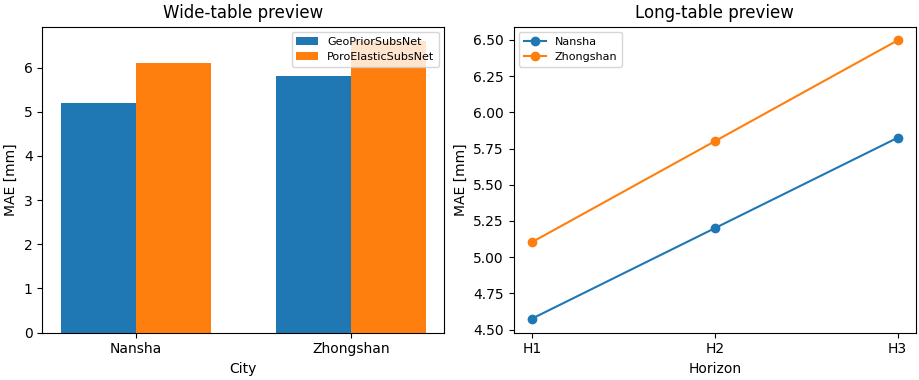
Build one compact visual preview#
This preview is not part of the production builder itself. It is a teaching aid for the gallery page.
- Left:
city/model MAE summary from the wide table.
- Right:
horizon-level MAE drift for GeoPriorSubsNet from the long table.
city_model = (
    wide.groupby(["city", "model"], as_index=False)["mae"]
    .mean()
    .sort_values(["city", "model"])
)

geo_long = long.loc[
    long["model"] == "GeoPriorSubsNet"
].copy()
geo_long["horizon_n"] = geo_long["horizon"].str.replace(
    "H",
    "",
    regex=False,
).astype(int)

fig, axes = plt.subplots(
    1,
    2,
    figsize=(9.2, 3.8),
    constrained_layout=True,
)

# Grouped city/model bar view
ax = axes[0]
cities = list(dict.fromkeys(city_model["city"]))
models = list(dict.fromkeys(city_model["model"]))
x = np.arange(len(cities))
w = 0.35

for i, model in enumerate(models):
    vals = []
    for city in cities:
        sub = city_model.loc[
            (city_model["city"] == city)
            & (city_model["model"] == model),
            "mae",
        ]
        vals.append(float(sub.iloc[0]) if not sub.empty else np.nan)

    ax.bar(
        x + (i - 0.5) * w,
        vals,
        width=w,
        label=model,
    )

ax.set_title("Wide-table preview")
ax.set_xlabel("City")
ax.set_ylabel("MAE [mm]")
ax.set_xticks(x)
ax.set_xticklabels(cities)
ax.legend(fontsize=8)

# Horizon drift view
ax = axes[1]
for city in sorted(geo_long["city"].dropna().unique()):
    sub = geo_long.loc[
        geo_long["city"] == city
    ].sort_values("horizon_n")

    ax.plot(
        sub["horizon_n"].to_numpy(),
        sub["mae"].to_numpy(),
        marker="o",
        label=city,
    )

ax.set_title("Long-table preview")
ax.set_xlabel("Horizon")
ax.set_ylabel("MAE [mm]")
ax.set_xticks([1, 2, 3])
ax.set_xticklabels(["H1", "H2", "H3"])
ax.legend(fontsize=8)
<matplotlib.legend.Legend object at 0x749e55c26b70>
Learn how to read the wide table#
The wide table is the run archive.
A practical reading order is:
identify the run descriptors such as timestamp, city, model, PDE mode, and lambda weights;
read the headline metrics such as MAE, RMSE, R2, coverage80, sharpness80, epsilon_prior, and epsilon_cons;
inspect the expanded interval-calibration fields only when you need to compare calibrated versus uncalibrated uncertainty.
In other words:
the wide table is the archive for run-level comparison,
the long table is the archive for horizon-level comparison.
Learn how to read the long table#
The long table is useful when the question is not:
“Which run is best overall?”
but instead:
“How does performance drift across forecast horizons?”
Each long-table row keeps the run identity columns and adds:
one horizon label,
horizon-specific R2,
horizon-specific MAE,
optional pre/post calibration interval metrics.
That makes it very easy to:
plot horizon trajectories,
compute horizon averages,
or compare calibration effects by step.
Why deduplication matters#
In this lesson, the Nansha + GeoPrior run was intentionally written twice:
once as a legacy record,
once as an updated record.
The builder prefers updated records and then deduplicates by
(timestamp, city, model).
That is important in real workflows because re-runs or patched exports often leave multiple JSONL files on disk for the same logical experiment.
Why interval calibration fields are useful#
When interval-calibration diagnostics are present in the ablation record, the builder exports them into flat columns.
That matters because it turns a deeply nested JSON block into something directly usable in:
CSV audits,
spreadsheet summaries,
or quick plots like the horizon-calibration view above.
Command-line version#
The same lesson can be reproduced from the CLI.
Legacy dispatcher:
python -m scripts build-model-metrics \
  --src results \
  --out model_metrics \
  --include-long true
Modern CLI:
geoprior build model-metrics \
  --src results \
  --out model_metrics \
  --include-long true
With filters:
geoprior build model-metrics \
  --src results \
  --city Nansha,Zhongshan \
  --models GeoPriorSubsNet \
  --dedupe true \
  --include-long true
The gallery page teaches the builder. The command line reproduces it in a workflow.
Total running time of the script: (0 minutes 0.261 seconds)