
Note
Go to the end to download the full example code.
Inspect a model-initialization manifest before training#
This lesson explains how to inspect the
model_init_manifest.json artifact.
Why this artifact matters#
The model-initialization manifest is one of the most useful files to read before a long training run starts. It sits between Stage-1 preprocessing and Stage-2 optimization and answers practical questions such as:
Which model class was actually initialized?
What input and output dimensions will the model expect?
Which architecture choices were resolved?
Which GeoPrior physics knobs were activated at initialization?
Which scaling conventions and feature-channel identities were already frozen into the model configuration?
This matters because a training job can fail, or worse, run successfully with the wrong assumptions, even when the data files themselves are fine. A mismatch in feature counts, quantile setup, coordinate conventions, forcing interpretation, or physics initialization can change the entire meaning of the run.
What this lesson teaches#
We will use the inspection layer as a reading guide:
build a realistic initialization manifest,
load it through the standard inspection API,
read the compact semantic summary,
inspect model dimensions,
inspect architecture and sequence-design choices,
inspect GeoPrior initialization knobs,
inspect the resolved scaling overview,
inspect feature-group identities,
end with a compact decision rule.
This is intentionally a teaching page, not only an API demo. After most sections, we explain what the view means, why it matters, and what would count as a warning sign in a real workflow.
from __future__ import annotations

import tempfile
from pathlib import Path
from pprint import pprint

import matplotlib.pyplot as plt
import pandas as pd

from geoprior.utils.inspect import (
    generate_model_init_manifest,
    inspect_model_init_manifest,
    load_model_init_manifest,
    model_init_architecture_frame,
    model_init_dims_frame,
    model_init_feature_groups_frame,
    model_init_geoprior_frame,
    model_init_scaling_overview_frame,
    plot_model_init_architecture,
    plot_model_init_boolean_summary,
    plot_model_init_dims,
    plot_model_init_feature_group_sizes,
    plot_model_init_geoprior,
    summarize_model_init_manifest,
)

pd.set_option("display.max_columns", 24)
pd.set_option("display.width", 110)


MODEL_INIT_PALETTE = {
    "dims": "#2563EB",
    "arch": "#9333EA",
    "geoprior": "#EA580C",
    "features": "#0F766E",
    "pass": "#15803D",
    "fail": "#B91C1C",
    "edge": "#312E81",
    "panel": "#FCFCFF",
}


def _style_bar_panel(
    ax: plt.Axes,
    *,
    color: str,
    edge: str | None = None,
) -> None:
    """Polish a bar-based gallery panel."""
    edge = edge or MODEL_INIT_PALETTE["edge"]
    for patch in ax.patches:
        patch.set_facecolor(color)
        patch.set_edgecolor(edge)
        patch.set_linewidth(1.25)
        patch.set_alpha(0.94)
    ax.set_facecolor(MODEL_INIT_PALETTE["panel"])
    ax.tick_params(labelsize=9)
    ax.title.set_fontweight("bold")
    for side in ("top", "right"):
        ax.spines[side].set_visible(False)
    for side in ("left", "bottom"):
        ax.spines[side].set_color("#CBD5E1")


def _style_boolean_panel(ax: plt.Axes) -> None:
    """Apply a distinct pass/fail palette to boolean panels."""
    for patch in ax.patches:
        width = patch.get_width()
        height = patch.get_height()
        score = width if width != 0 else height
        color = (
            MODEL_INIT_PALETTE["pass"]
            if score >= 0.5
            else MODEL_INIT_PALETTE["fail"]
        )
        patch.set_facecolor(color)
        patch.set_edgecolor(MODEL_INIT_PALETTE["edge"])
        patch.set_linewidth(1.15)
        patch.set_alpha(0.94)
    ax.set_facecolor(MODEL_INIT_PALETTE["panel"])
    ax.tick_params(labelsize=9)
    ax.title.set_fontweight("bold")
    for side in ("top", "right"):
        ax.spines[side].set_visible(False)
    for side in ("left", "bottom"):
        ax.spines[side].set_color("#CBD5E1")
Create a realistic demo artifact#
For a gallery lesson, we usually want a deterministic artifact rather than rebuilding a full model. The generation helper gives us a stable initialization manifest with the same broad structure as a real one.
Here we make a few choices explicit so the lesson becomes easier to interpret:
a non-trivial forecast horizon,
a real quantile set,
an explicit PDE mode,
an identifiability regime,
and a scaling payload that still carries rich physics metadata.
The goal is not to claim that this is the only correct setup. The goal is to create a realistic manifest that teaches how to inspect one.
workdir = Path(tempfile.mkdtemp(prefix="gp_sg_model_init_"))
json_path = workdir / "demo_model_init_manifest.json"

_ = generate_model_init_manifest(
    json_path,
    overrides={
        "model_class": "GeoPriorSubsNet",
        "dims": {
            "forecast_horizon": 3,
            "static_input_dim": 12,
            "dynamic_input_dim": 5,
            "future_input_dim": 1,
            "output_subsidence_dim": 1,
            "output_gwl_dim": 1,
        },
        "config": {
            "mode": "tft_like",
            "pde_mode": "on",
            "identifiability_regime": "anchored",
            "quantiles": [0.1, 0.5, 0.9],
            "embed_dim": 48,
            "hidden_units": 96,
            "lstm_units": 96,
            "attention_units": 64,
            "num_heads": 4,
            "memory_size": 64,
            "dropout_rate": 0.1,
            "geoprior": {
                "hd_factor": 0.5,
                "use_effective_h": True,
                "offset_mode": "mul",
                "kappa_mode": "kb",
            },
            "scaling_kwargs": {
                "coords_normalized": True,
                "coord_ranges": {"t": 7.0, "x": 44447.0, "y": 39275.0},
                "Q_kind": "per_volume",
                "mv_weight": 0.001,
                "mv_schedule_unit": "epoch",
                "mv_delay_epochs": 1,
                "mv_warmup_epochs": 2,
                "track_aux_metrics": True,
            },
        },
    },
)

print("Written artifact:")
print(f" - {json_path}")
Written artifact:
 - /tmp/gp_sg_model_init_x8oynglk/demo_model_init_manifest.json
Load the artifact through the inspection layer#
The loader returns a small artifact record so later utilities can work consistently with either a path, a mapping, or an already loaded payload.
In a real workflow, this is the same entry point you would use when a
training preparation step has already written
model_init_manifest.json.
record = load_model_init_manifest(json_path)
payload = record.payload

print("Artifact kind:", record.kind)
print("Artifact path:", record.path)
Artifact kind: model_init_manifest
Artifact path: /tmp/gp_sg_model_init_x8oynglk/demo_model_init_manifest.json
Read the compact summary first#
The summary is the fastest way to answer the first inspection question:
What kind of model did we really initialize?
This is a better starting point than opening the whole JSON because it condenses the most decision-relevant items:
model class,
input and output dimensions,
architecture mode,
quantile count,
PDE mode,
identifiability regime,
coordinate and groundwater conventions,
feature-group counts,
and the presence of physical bounds.
{'coord_order': ['t', 'x', 'y'],
 'coords_in_degrees': False,
 'coords_normalized': True,
 'dynamic_input_dim': 5,
 'forecast_horizon': 3,
 'future_input_dim': 1,
 'gamma_w': 9810.0,
 'gwl_kind': 'depth_bgs',
 'gwl_sign': 'down_positive',
 'hd_factor': 0.5,
 'identifiability_regime': 'anchored',
 'init_kappa': 1.0,
 'init_mv': 1e-07,
 'kappa_mode': 'kb',
 'mode': 'tft_like',
 'model_class': 'GeoPriorSubsNet',
 'mv_prior_mode': 'calibrate',
 'mv_schedule_unit': 'epoch',
 'n_bounds': 14,
 'n_dynamic_features': 5,
 'n_future_features': 1,
 'n_static_features': 12,
 'offset_mode': 'mul',
 'output_gwl_dim': 1,
 'output_subsidence_dim': 1,
 'pde_mode': 'on',
 'q_kind': 'per_volume',
 'quantile_count': 3,
 'quantiles': [0.1, 0.5, 0.9],
 'static_input_dim': 12,
 'time_units': 'year',
 'use_batch_norm': False,
 'use_effective_h': True,
 'use_head_proxy': True,
 'use_residuals': True,
 'use_vsn': True}
How to interpret the summary#
When I inspect an initialization manifest, I usually read the summary in this order:
Model identity
model_classtells you which family was built. This matters if your workflow can initialize different model variants.Dimension contract
static_input_dim,dynamic_input_dim, andfuture_input_dimdefine the input interface the model expects. These numbers should be compatible with the exported Stage-1 feature groups.Forecast meaning
forecast_horizonplusquantilesdetermine the semantic shape of the outputs. A mismatch here changes not only tensor shapes, but also the meaning of the prediction head.Physics and identifiability setup
pde_mode,identifiability_regime,q_kind,mv_prior_mode, anduse_effective_htell you how much physics is switched on and how strongly the initialization is constrained.Scaling convention
coords_normalized,coords_in_degrees,gwl_kind, andgwl_signtell you whether the geometry and groundwater channels will be interpreted the way you think they will.
A useful mental model is this: the summary is not yet a deep audit, but it is the best place to catch obvious mismatches before you inspect the detailed tables.
Inspect the dimension contract as a table#
The dimensions table answers a concrete engineering question:
What tensor shapes is this model prepared to receive and emit?
In practice, these dimensions should agree with the Stage-1 preprocessing outputs. If they do not, a training run may fail immediately, or may pass shape checks while still learning from a misinterpreted feature layout.
dims_frame = model_init_dims_frame(payload)
print(dims_frame.to_string(index=False))
section                  name  value
   dims     dynamic_input_dim      5
   dims      forecast_horizon      3
   dims      future_input_dim      1
   dims        output_gwl_dim      1
   dims output_subsidence_dim      1
   dims      static_input_dim     12
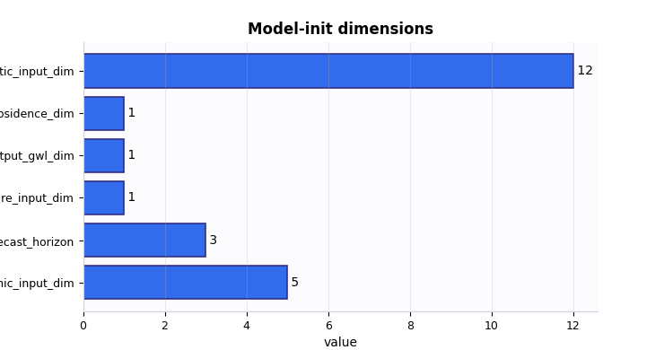
Plot 1: model dimensions#
This plot turns the input/output dimension contract into a compact view. It is especially useful when teaching new users how the architecture sees the data.
How to read it:
the three input bars tell you how wide each feature family is,
forecast_horizontells you how many future steps the model will emit,the two output bars show whether you are predicting both subsidence and groundwater or only one target family.
What would be suspicious?
a zero-sized future input when the workflow claims future-known drivers are enabled,
an unexpected output dimension,
or feature counts that do not match the preprocessing manifest.
fig, ax = plt.subplots(figsize=(7.4, 3.9))
plot_model_init_dims(
    payload,
    ax=ax,
)
_style_bar_panel(ax, color=MODEL_INIT_PALETTE["dims"])
plt.show()
Inspect architecture choices as a table#
The architecture table is where we move from data contract to model design. It tells us how much capacity and sequence-processing machinery the run was initialized with.
This matters because two runs can share the same data files but still be very different models if they resolve different attention widths, recurrent sizes, or sequence memory depth.
arch_frame = model_init_architecture_frame(payload)
print(arch_frame.to_string(index=False))
     section                    key           value
architecture              embed_dim              48
architecture           hidden_units              96
architecture             lstm_units              96
architecture        attention_units              64
architecture              num_heads               4
architecture           dropout_rate        0.100000
architecture            memory_size              64
architecture              vsn_units              32
architecture                   mode        tft_like
architecture               pde_mode              on
architecture identifiability_regime        anchored
architecture              quantiles [0.1, 0.5, 0.9]
architecture                 scales          [1, 2]
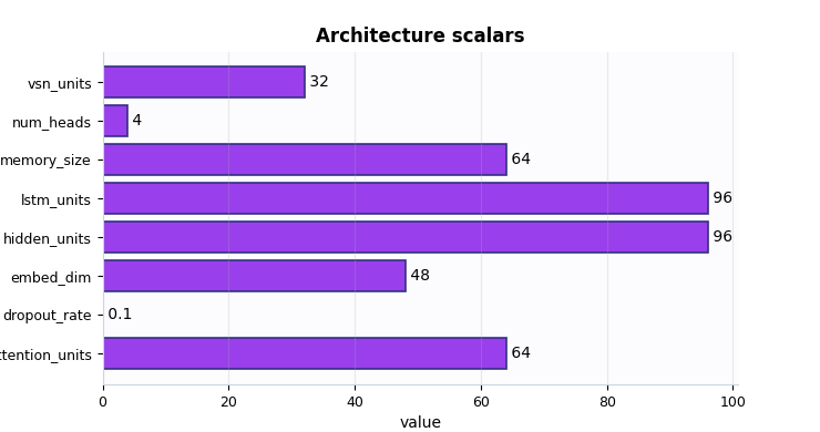
Plot 2: architecture scalars#
This plot is not trying to prove that one architecture is better than another. Its purpose is to help the user understand the scale of the initialized model.
A good reading strategy is:
compare
embed_dimandhidden_unitsto understand the internal width of the representation,compare
lstm_unitsandmemory_sizeto understand how much temporal capacity was requested,look at
num_headsandattention_unitsto see whether attention is lightweight or relatively expressive,check whether
dropout_rateis close to your expectation.
A warning sign is not simply “large” or “small”. A warning sign is a design that contradicts the training intention. For example, a tiny memory size with a long sequence task, or quantile forecasting with a head layout you did not intend.
fig, ax = plt.subplots(figsize=(7.4, 3.9))
plot_model_init_architecture(
    payload,
    ax=ax,
)
_style_bar_panel(ax, color=MODEL_INIT_PALETTE["arch"])
plt.show()
Inspect GeoPrior initialization knobs#
The geoprior block is the most physics-specific part of the
initialization manifest. It tells us how the model was anchored before
any gradient update happened.
This block is important because it encodes choices that strongly affect stability and identifiability later:
gamma_wsets the unit-weight-of-water convention,h_ref_modeandh_ref_valuecontrol the reference-head setup,hd_factoranduse_effective_hinfluence the effective drainage thickness used by closures,init_kappaandinit_mvdetermine the starting scale for key physical parameters,offset_modeandkappa_modetell you how the physics terms are parameterized.
geoprior_frame = model_init_geoprior_frame(payload)
print(geoprior_frame.to_string(index=False))
 section             key       value
geoprior         gamma_w 9810.000000
geoprior     h_ref_value    0.000000
geoprior       hd_factor    0.500000
geoprior      init_kappa    1.000000
geoprior         init_mv    0.000000
geoprior      h_ref_mode        auto
geoprior      kappa_mode          kb
geoprior     offset_mode         mul
geoprior use_effective_h        True
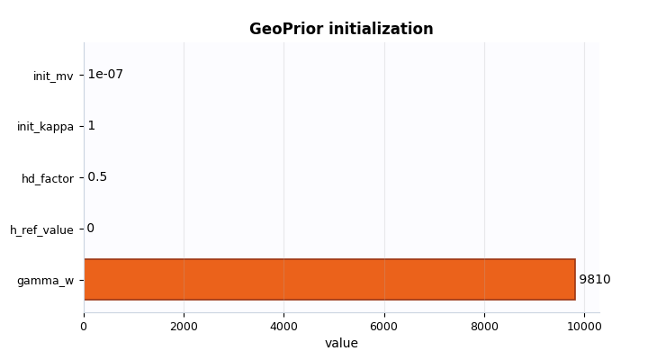
Plot 3: GeoPrior initialization scalars#
This plot condenses the most numeric part of the GeoPrior initialization. I usually read it as a physics readiness view.
In particular:
hd_factortells you whether effective thickness is being damped,init_kappaandinit_mvtell you where the learnable physics parameters start,gamma_whelps confirm the unit convention,and
h_ref_valuetells you whether a fixed non-zero reference was injected at initialization.
A suspicious pattern here would be an implausible combination such as a strong effective-thickness assumption with a completely unexpected reference-head policy or starting values far from the intended regime.
fig, ax = plt.subplots(figsize=(7.4, 3.9))
plot_model_init_geoprior(
    payload,
    ax=ax,
)
_style_bar_panel(ax, color=MODEL_INIT_PALETTE["geoprior"], edge="#9A3412")
plt.show()
Inspect the resolved scaling overview#
Even though this is an initialization artifact, it already carries a
resolved scaling_kwargs view. That is extremely valuable because the
model is not initialized in isolation: it is initialized together with
coordinate conventions, units, forcing interpretation, schedules, and
bounds.
In other words, this table is where architecture and physical semantics meet.
scaling_frame = model_init_scaling_overview_frame(payload)
print(scaling_frame.head(28).to_string(index=False))
         section                   key           value
scaling_overview            time_units            year
scaling_overview seconds_per_time_unit 31556952.000000
scaling_overview     coords_normalized            True
scaling_overview     coords_in_degrees           False
scaling_overview       coord_epsg_used           32649
scaling_overview        coord_src_epsg            4326
scaling_overview     coord_target_epsg           32649
scaling_overview      clip_global_norm        5.000000
scaling_overview   cons_residual_units          second
scaling_overview     gw_residual_units          second
scaling_overview      cons_scale_floor        0.000000
scaling_overview        gw_scale_floor        0.000000
scaling_overview                Q_kind      per_volume
scaling_overview               Q_in_si           False
scaling_overview       Q_in_per_second           False
scaling_overview        Q_length_in_si           False
scaling_overview Q_wrt_normalized_time           False
scaling_overview              lambda_q        0.000500
scaling_overview             mv_weight        0.001000
scaling_overview      mv_schedule_unit           epoch
scaling_overview       mv_delay_epochs               1
scaling_overview      mv_warmup_epochs               2
scaling_overview    physics_ramp_steps             500
scaling_overview  physics_warmup_steps             500
    coord_ranges         coord_range_t        7.000000
    coord_ranges         coord_range_x    44447.000000
    coord_ranges         coord_range_y    39275.000000
   bounds_config           bounds_mode            soft
How to read the scaling overview#
A user does not need to memorize every key in this table. A better strategy is to scan it by themes:
- Geometry and units
time_units,coords_normalized,coords_in_degrees, and the coordinate EPSG keys tell you how the derivative geometry will be interpreted.- Residual conventions
cons_residual_unitsandgw_residual_unitstell you in which unit family the residuals are expected to live.- Forcing interpretation
Q_kindplus theQ_*flags tell you whether the forcing term is interpreted as per-volume forcing, a length rate, or some other convention.- Regularization schedules
mv_weight,mv_schedule_unit, delay, and warmup keys tell you how strongly the MV prior enters and when.- Bounds policy
The nested
bounds_*rows tell you whether the initialization is already carrying a bounded physics design.
A real warning sign is not “many keys”. It is inconsistency across these
themes. For example: normalized coordinates without plausible ranges,
forcing flags that contradict Q_kind, or a strong prior schedule that
the training plan did not expect.
Inspect feature-group identities#
The feature-group table answers a very practical question:
Which columns does the initialized model believe belong to each input family?
This is often more important than the dimension counts themselves. A run can have the correct width but still have the wrong feature order.
In particular, the dynamic group is worth reading carefully because it defines channel identities such as groundwater and subsidence drivers.
feature_frame = model_init_feature_groups_frame(payload)
print(feature_frame.head(24).to_string(index=False))
  group  index                        feature_name
 static      0    lithology_Conglomerate–Sandstone
 static      1       lithology_Limestone–Sandstone
 static      2        lithology_Mudstone–Siltstone
 static      3       lithology_Sandstone–Siltstone
 static      4           lithology_Shale–Limestone
 static      5       lithology_Siltstone–Sandstone
 static      6           lithology_Siltstone–Shale
 static      7            lithology_Tuff–Sandstone
 static      8 lithology_class_Coarse-Grained Soil
 static      9   lithology_class_Fine-Grained Soil
 static     10      lithology_class_Mixed Clastics
 static     11                        z_surf_m__si
dynamic      0                 GWL_depth_bgs_m__si
dynamic      1                  subsidence_cum__si
dynamic      2                         rainfall_mm
dynamic      3                   urban_load_global
dynamic      4             soil_thickness_censored
 future      0                         rainfall_mm
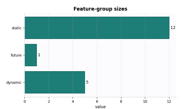
Plot 4: feature-group sizes#
This plot is simple, but it is pedagogically useful. It gives a very fast picture of how the initialized model distributes information across static, dynamic, and future-known inputs.
How to interpret it:
a larger static group suggests a stronger role for site/context encoding,
a larger dynamic group suggests a richer sequential input stream,
a non-empty future group confirms the model expects future-known drivers.
A suspicious pattern would be an empty future group when the intended workflow depends on future rainfall or other future-known covariates.
fig, ax = plt.subplots(figsize=(6.8, 3.8))
plot_model_init_feature_group_sizes(
    payload,
    ax=ax,
)
_style_bar_panel(ax, color=MODEL_INIT_PALETTE["features"], edge="#115E59")
plt.show()
Use the all-in-one inspector#
Once the main sections look plausible, the all-in-one inspector is a good way to consolidate the reading. It returns:
the compact summary,
tidy frames for dimensions, architecture, GeoPrior, scaling, and feature groups,
a flattened key-value view,
and optional figure paths if you ask it to save plots.
This is often the most practical entry point for later CLI-based folder inspection, report generation, or debugging notebooks.
bundle_dir = workdir / "inspection_bundle"
bundle = inspect_model_init_manifest(
    payload,
    output_dir=bundle_dir,
    stem="lesson_model_init",
    save_figures=True,
)

print("Bundle keys:")
print(sorted(bundle))
print("Frame keys:")
print(sorted(bundle["frames"]))
print("Saved figures:")
for name, path in bundle["figure_paths"].items():
    print(f" - {name}: {path}")
Bundle keys:
['figure_paths', 'frames', 'summary']
Frame keys:
['architecture', 'dims', 'feature_groups', 'flattened', 'geoprior', 'scaling_overview']
Saved figures:
 - lesson_model_init_dims.png: /tmp/gp_sg_model_init_x8oynglk/inspection_bundle/lesson_model_init_dims.png
 - lesson_model_init_architecture.png: /tmp/gp_sg_model_init_x8oynglk/inspection_bundle/lesson_model_init_architecture.png
 - lesson_model_init_geoprior.png: /tmp/gp_sg_model_init_x8oynglk/inspection_bundle/lesson_model_init_geoprior.png
 - lesson_model_init_feature_groups.png: /tmp/gp_sg_model_init_x8oynglk/inspection_bundle/lesson_model_init_feature_groups.png
 - lesson_model_init_checks.png: /tmp/gp_sg_model_init_x8oynglk/inspection_bundle/lesson_model_init_checks.png
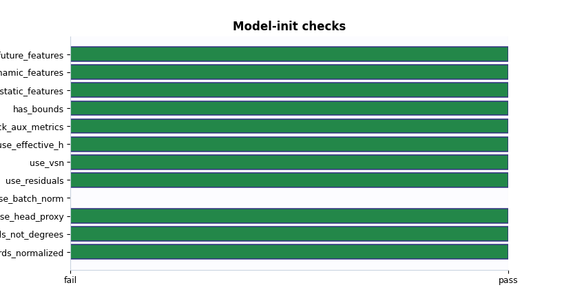
Plot 5: compact boolean checks#
The boolean summary is the fastest decision view on this page. It intentionally compresses the initialization state into a small set of checks such as:
coordinates normalized,
coordinates not left in raw degrees,
head proxy active,
residual and VSN paths enabled,
effective thickness active,
feature groups present,
bounds present.
This is not a substitute for the earlier tables. It is the final quick screen you can use before saying “this looks ready enough to train”.
A practical decision rule#
For this artifact family, a simple and useful decision rule is:
the model class is the one you intended,
input/output dimensions look compatible with Stage-1,
quantiles and forecast horizon match the task,
the GeoPrior initialization block matches the physics plan,
scaling conventions are plausible,
bounds are present when the run is meant to use bounded physics,
static, dynamic, and future feature groups all look healthy.
If these conditions are satisfied, the model-init manifest usually looks trustworthy enough to proceed to training and later evaluation.
must_hold = [
    summary.get("model_class") == "GeoPriorSubsNet",
    int(summary.get("static_input_dim") or 0) > 0,
    int(summary.get("dynamic_input_dim") or 0) > 0,
    int(summary.get("future_input_dim") or 0) > 0,
    int(summary.get("forecast_horizon") or 0) > 0,
    int(summary.get("quantile_count") or 0) > 0,
    bool(summary.get("coords_normalized")),
    not bool(summary.get("coords_in_degrees")),
    int(summary.get("n_bounds") or 0) > 0,
    bool(summary.get("use_effective_h")),
]

print("\nDecision note")
if all(must_hold):
    print(
        "This demo model-init manifest looks structurally ready "
        "for Stage-2 training."
    )
else:
    print(
        "This initialization manifest needs attention before "
        "training begins."
    )
Decision note
This demo model-init manifest looks structurally ready for Stage-2 training.
Total running time of the script: (0 minutes 0.987 seconds)