Note

Go to the end to download the full example code.

Stage-2 training curves and physics diagnostics#

This lesson teaches how to read training-history curves during Stage-2 model fitting.

Why this page matters#

A model can produce a decreasing training loss and still be scientifically unstable.

For GeoPrior-style training, it is rarely enough to look only at:

loss
val_loss

because the training loop can also expose physics-aware quantities such as:

data_loss
physics_loss or physics_loss_scaled
physics_mult
lambda_offset
consolidation_loss
gw_flow_loss
prior_loss
smooth_loss
mv_prior_loss
bounds_loss
epsilon_prior
epsilon_cons
epsilon_gw

Those names are not invented for this lesson: they come directly from the model’s logging surface and physics bundle packaging. GeoPrior also registers epsilon_prior, epsilon_cons, and epsilon_gw as tracked metrics, and its physics evaluator aggregates scalar keys whose names begin with loss_ or epsilon_.

What this lesson teaches#

We will:

build a compact synthetic history table that mimics a Stage-2 run,
inspect the real log names GeoPrior users should expect,
plot loss curves,
plot physics residual curves,
plot warmup / scaling controls such as physics_mult,
explain how to interpret stable versus unstable training behavior.

This page uses synthetic values so it is fully executable during the documentation build, but the column names and diagnostic logic are grounded in the real GeoPrior training/evaluation surface. :contentReference[oaicite:7]{index=7}

Imports#

We use plain pandas + matplotlib here because the files you shared do not expose a dedicated public helper specifically for Stage-2 training curves. The lesson therefore focuses on the real log keys and how to interpret them.

from __future__ import annotations

import numpy as np
import pandas as pd
import matplotlib.pyplot as plt

Step 1 - Build a compact synthetic training history#

We mimic a Stage-2 run over 60 epochs.

The synthetic curves are designed to illustrate a realistic training story:

total loss decreases,
validation loss improves and then plateaus,
physics pressure ramps in gradually,
epsilon diagnostics fall but not identically,
one component shows mild late instability.

The key point is that the column names match the kinds of metrics GeoPrior actually logs during training. :contentReference[oaicite:8]{index=8}

rng = np.random.default_rng(19)

epochs = np.arange(1, 61)

# Core supervised losses
data_loss = (
    1.15 * np.exp(-epochs / 18.0)
    + 0.07
    + rng.normal(0.0, 0.008, size=epochs.size)
)

# Physics warmup / multiplier ramp
physics_mult = np.clip((epochs - 8) / 18.0, 0.0, 1.0)

# Offset / weighting control
lambda_offset = np.clip(0.25 + 0.018 * epochs, 0.25, 1.0)

# Physics components
consolidation_loss = (
    0.50 * np.exp(-epochs / 14.0)
    + 0.03
    + rng.normal(0.0, 0.005, size=epochs.size)
)

gw_flow_loss = (
    0.44 * np.exp(-epochs / 16.0)
    + 0.04
    + rng.normal(0.0, 0.005, size=epochs.size)
)

prior_loss = (
    0.35 * np.exp(-epochs / 20.0)
    + 0.025
    + rng.normal(0.0, 0.004, size=epochs.size)
)

smooth_loss = (
    0.12 * np.exp(-epochs / 25.0)
    + 0.012
    + rng.normal(0.0, 0.002, size=epochs.size)
)

mv_prior_loss = (
    0.05 * np.exp(-epochs / 17.0)
    + 0.006
    + rng.normal(0.0, 0.0012, size=epochs.size)
)

bounds_loss = (
    0.08 * np.exp(-epochs / 11.0)
    + 0.005
    + rng.normal(0.0, 0.0015, size=epochs.size)
)

physics_loss_raw = (
    consolidation_loss
    + gw_flow_loss
    + prior_loss
    + smooth_loss
    + mv_prior_loss
    + bounds_loss
)

physics_loss_scaled = physics_mult * (
    consolidation_loss
    + gw_flow_loss
    + prior_loss
    + smooth_loss
    + bounds_loss
) + mv_prior_loss

# Total loss surface
loss = data_loss + physics_loss_scaled
total_loss = loss.copy()

# Validation curves
val_loss = (
    1.05 * np.exp(-epochs / 17.0)
    + 0.11
    + 0.0009 * np.maximum(epochs - 36, 0)
    + rng.normal(0.0, 0.010, size=epochs.size)
)

# Epsilon-style diagnostics
epsilon_prior = (
    0.52 * np.exp(-epochs / 16.0)
    + 0.045
    + rng.normal(0.0, 0.006, size=epochs.size)
)
epsilon_cons = (
    0.48 * np.exp(-epochs / 18.0)
    + 0.050
    + 0.0012 * np.maximum(epochs - 42, 0)
    + rng.normal(0.0, 0.006, size=epochs.size)
)
epsilon_gw = (
    0.42 * np.exp(-epochs / 15.0)
    + 0.055
    + rng.normal(0.0, 0.006, size=epochs.size)
)

# Optional validation epsilon diagnostics for teaching
val_epsilon_prior = epsilon_prior + 0.02 + rng.normal(
    0.0,
    0.005,
    size=epochs.size,
)
val_epsilon_cons = epsilon_cons + 0.025 + rng.normal(
    0.0,
    0.006,
    size=epochs.size,
)
val_epsilon_gw = epsilon_gw + 0.02 + rng.normal(
    0.0,
    0.006,
    size=epochs.size,
)

history_df = pd.DataFrame(
    {
        "epoch": epochs,
        "loss": loss,
        "total_loss": total_loss,
        "val_loss": val_loss,
        "data_loss": data_loss,
        "physics_loss": physics_loss_raw,
        "physics_loss_scaled": physics_loss_scaled,
        "physics_mult": physics_mult,
        "lambda_offset": lambda_offset,
        "consolidation_loss": consolidation_loss,
        "gw_flow_loss": gw_flow_loss,
        "prior_loss": prior_loss,
        "smooth_loss": smooth_loss,
        "mv_prior_loss": mv_prior_loss,
        "bounds_loss": bounds_loss,
        "epsilon_prior": epsilon_prior,
        "epsilon_cons": epsilon_cons,
        "epsilon_gw": epsilon_gw,
        "val_epsilon_prior": val_epsilon_prior,
        "val_epsilon_cons": val_epsilon_cons,
        "val_epsilon_gw": val_epsilon_gw,
    }
)

print("History table shape:", history_df.shape)
print("")
print(history_df.head(10).to_string(index=False))

History table shape: (60, 21)

 epoch     loss  total_loss  val_loss  data_loss  physics_loss  physics_loss_scaled  physics_mult  lambda_offset  consolidation_loss  gw_flow_loss  prior_loss  smooth_loss  mv_prior_loss  bounds_loss  epsilon_prior  epsilon_cons  epsilon_gw  val_epsilon_prior  val_epsilon_cons  val_epsilon_gw
1.207225    1.207225  1.109575   1.154893      1.568382             0.052332      0.000000          0.268            0.497382      0.452886    0.358390     0.125282       0.052332     0.082111       0.533422      0.485662    0.444566           0.552568          0.514674        0.468529
1.157243    1.157243  1.039216   1.107018      1.477249             0.050225      0.000000          0.286            0.468932      0.424404    0.342694     0.121089       0.050225     0.069906       0.500421      0.477095    0.414776           0.525079          0.509243        0.439319
1.093349    1.093349  0.979611   1.046781      1.396053             0.046568      0.000000          0.304            0.436299      0.407846    0.321640     0.116445       0.046568     0.067256       0.470000      0.445381    0.410633           0.480971          0.472841        0.428650
1.032538    1.032538  0.945322   0.985903      1.320559             0.046635      0.000000          0.322            0.408028      0.373508    0.314814     0.116695       0.046635     0.060880       0.441409      0.425112    0.378401           0.465841          0.454723        0.398503
0.989945    0.989945  0.885284   0.946462      1.254167             0.043483      0.000000          0.340            0.377581      0.364324    0.303083     0.108476       0.043483     0.057219       0.425722      0.404059    0.365498           0.443103          0.438774        0.383663
0.924755    0.924755  0.866464   0.882411      1.185074             0.042344      0.000000          0.358            0.349540      0.347184    0.284044     0.107034       0.042344     0.054928       0.404275      0.385900    0.339306           0.416110          0.411642        0.372273
0.893282    0.893282  0.804780   0.854229      1.123618             0.039053      0.000000          0.376            0.337996      0.319068    0.275827     0.103995       0.039053     0.047679       0.385218      0.369207    0.319456           0.407070          0.389109        0.334567
0.839238    0.839238  0.771813   0.802863      1.076260             0.036376      0.000000          0.394            0.315391      0.314227    0.263494     0.101879       0.036376     0.044893       0.355465      0.356204    0.307394           0.377600          0.375199        0.331509
0.861855    0.861855  0.719305   0.772562      0.990665             0.089293      0.055556          0.412            0.283756      0.298366    0.237241     0.095231       0.036271     0.039800       0.345266      0.347851    0.289416           0.369983          0.377105        0.302440
0.868011    0.868011  0.697757   0.733329      0.954448             0.134682      0.111111          0.430            0.271185      0.278963    0.242652     0.091254       0.032211     0.038183       0.318284      0.328674    0.268492           0.341992          0.340573        0.292720

Step 2 - Inspect the available log keys#

Before plotting, it is good practice to inspect the history columns.

In a real run, this helps answer:

what did the training loop actually log?
which keys are supervised?
which keys are physics-aware?

GeoPrior’s training packers and metrics surface are designed to expose canonical fields like loss, total_loss, data_loss, physics-loss components, and epsilon-style diagnostics. :contentReference[oaicite:9]{index=9} :contentReference[oaicite:10]{index=10}

print("")
print("History columns")
print(history_df.columns.tolist())

History columns
['epoch', 'loss', 'total_loss', 'val_loss', 'data_loss', 'physics_loss', 'physics_loss_scaled', 'physics_mult', 'lambda_offset', 'consolidation_loss', 'gw_flow_loss', 'prior_loss', 'smooth_loss', 'mv_prior_loss', 'bounds_loss', 'epsilon_prior', 'epsilon_cons', 'epsilon_gw', 'val_epsilon_prior', 'val_epsilon_cons', 'val_epsilon_gw']

Step 3 - Plot total, validation, and data loss#

This is the first Stage-2 diagnostic every user looks at.

But the page deliberately keeps data_loss on the same panel, so users can distinguish:

the supervised fit term,
the total objective that also includes physics pressure,
the validation behavior.

fig, ax = plt.subplots(figsize=(8.4, 4.8))

ax.plot(
    history_df["epoch"],
    history_df["loss"],
    label="loss / total_loss",
)
ax.plot(
    history_df["epoch"],
    history_df["val_loss"],
    label="val_loss",
)
ax.plot(
    history_df["epoch"],
    history_df["data_loss"],
    label="data_loss",
)

ax.set_xlabel("Epoch")
ax.set_ylabel("Loss")
ax.set_title("Stage-2 training and validation loss")
ax.grid(True, linestyle=":", alpha=0.6)
ax.legend()

plt.tight_layout()
plt.show()

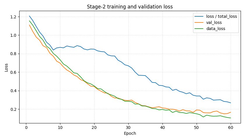
How to read the first panel#

`loss` and `total_loss`#

In GeoPrior logging, these are the authoritative optimization objectives. If they fall while data_loss rises badly, that may mean physics terms are dominating too strongly.

`val_loss`#

Validation loss is the first warning sign for overfitting or mismatch. A healthy training run often shows:

falling training loss,
falling validation loss,
then a plateau or mild divergence later.

`data_loss`#

This is the supervised fit term separated from physics regularization. It helps answer whether the model is improving the actual predictive fit or only reducing physics penalties.

Step 4 - Plot physics loss components#

The second essential panel separates the physics-aware objective.

GeoPrior’s training packers expose:

physics_loss or physics_loss_raw,
physics_loss_scaled,
and per-component terms such as consolidation_loss, gw_flow_loss, prior_loss, smooth_loss, mv_prior_loss, and bounds_loss.

fig, axes = plt.subplots(1, 2, figsize=(11.5, 4.4))

axes[0].plot(
    history_df["epoch"],
    history_df["physics_loss"],
    label="physics_loss",
)
axes[0].plot(
    history_df["epoch"],
    history_df["physics_loss_scaled"],
    label="physics_loss_scaled",
)
axes[0].set_xlabel("Epoch")
axes[0].set_ylabel("Physics objective")
axes[0].set_title("Raw vs scaled physics loss")
axes[0].grid(True, linestyle=":", alpha=0.6)
axes[0].legend()

for name in [
    "consolidation_loss",
    "gw_flow_loss",
    "prior_loss",
    "smooth_loss",
    "mv_prior_loss",
    "bounds_loss",
]:
    axes[1].plot(
        history_df["epoch"],
        history_df[name],
        label=name,
    )

axes[1].set_xlabel("Epoch")
axes[1].set_ylabel("Component loss")
axes[1].set_title("Physics-loss components")
axes[1].grid(True, linestyle=":", alpha=0.6)
axes[1].legend(fontsize=8)

plt.tight_layout()
plt.show()

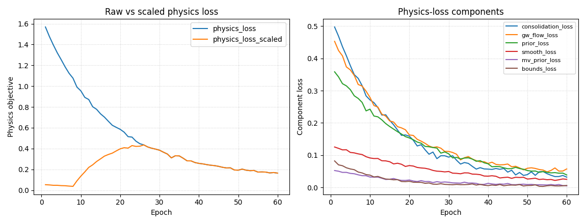
How to read the physics panel#

Raw vs scaled physics loss#

GeoPrior distinguishes the unscaled physics bundle from the scaled quantity that actually enters the total objective. That is why physics_loss and physics_loss_scaled can behave differently.

Component trends#

These curves tell you which part of the physics formulation is driving the run.

Useful quick interpretations:

falling prior_loss suggests the learned fields are moving toward the time-scale prior;
falling bounds_loss suggests fewer bound violations;
a stubborn gw_flow_loss may indicate unit, coordinate, or forcing mismatch;
a rising mv_prior_loss can indicate tension between storage structure and the data fit.

Step 5 - Plot epsilon diagnostics#

The model explicitly registers epsilon-style physics metrics:

epsilon_prior
epsilon_cons
epsilon_gw

These are meant as compact residual diagnostics, and the physics evaluator also treats epsilon_* as first-class aggregated scalar outputs.

fig, ax = plt.subplots(figsize=(8.8, 4.8))

for name in [
    "epsilon_prior",
    "epsilon_cons",
    "epsilon_gw",
    "val_epsilon_prior",
    "val_epsilon_cons",
    "val_epsilon_gw",
]:
    ax.plot(
        history_df["epoch"],
        history_df[name],
        label=name,
    )

ax.set_xlabel("Epoch")
ax.set_ylabel("Residual diagnostic")
ax.set_title("Epsilon-style physics diagnostics")
ax.grid(True, linestyle=":", alpha=0.6)
ax.legend(ncol=2, fontsize=9)

plt.tight_layout()
plt.show()

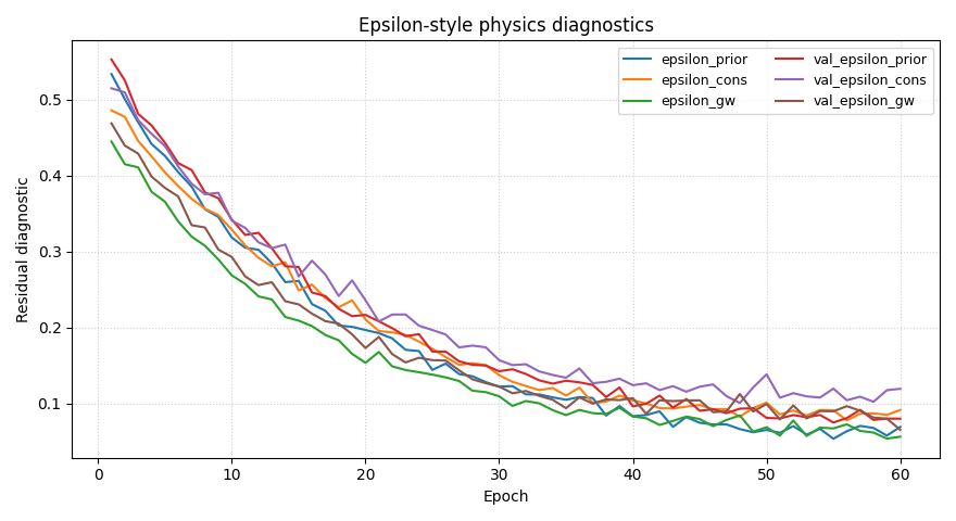
How to read the epsilon curves#

These are often the most scientifically informative curves in the page.

`epsilon_prior`#

Tracks mismatch against the time-scale prior / closure structure.

`epsilon_cons`#

Tracks consolidation consistency.

`epsilon_gw`#

Tracks groundwater-flow residual behavior.

A useful rule of thumb:

if all three fall together, the run is becoming more internally consistent;
if one stays flat while the others improve, that specific physics term may be the real bottleneck;
if a validation epsilon rises while the training epsilon falls, the physics fit may be becoming too specialized to the training set.

Step 6 - Plot warmup and scaling controls#

GeoPrior training can use warmup/ramp policies and offset-aware scaling. The documentation explicitly mentions training-policy fields such as physics_warmup_steps and physics_ramp_steps, and the training logs expose controls such as physics_mult and lambda_offset.

fig, ax = plt.subplots(figsize=(8.2, 4.6))

ax.plot(
    history_df["epoch"],
    history_df["physics_mult"],
    label="physics_mult",
)
ax.plot(
    history_df["epoch"],
    history_df["lambda_offset"],
    label="lambda_offset",
)

ax.set_xlabel("Epoch")
ax.set_ylabel("Control value")
ax.set_title("Physics warmup / offset controls")
ax.grid(True, linestyle=":", alpha=0.6)
ax.legend()

plt.tight_layout()
plt.show()

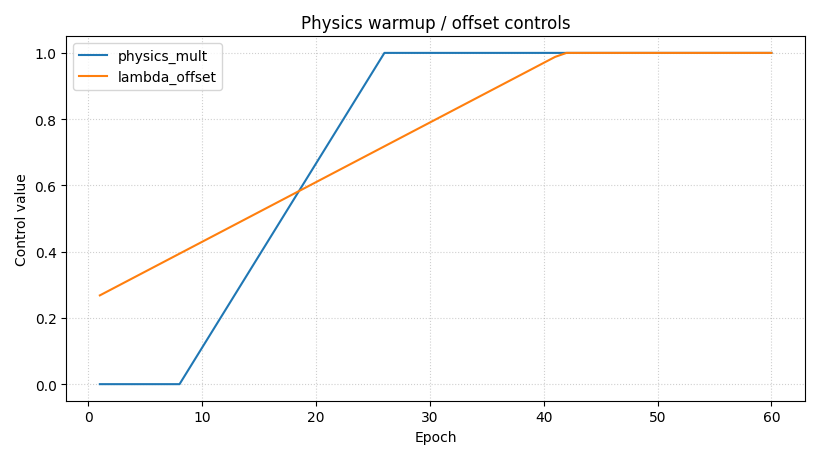
Why this control panel matters#

When training uses physics warmup or offset-aware scaling, a bad loss curve is not always a modeling failure. It may simply reflect that the physics term was activated gradually.

That is why this panel should be read before overreacting to a bump in loss or physics_loss_scaled.

Step 7 - Build a compact summary table#

A diagnostics page becomes more useful when the plots are paired with a small numerical summary.

summary = pd.DataFrame(
    [
        {
            "metric": "best_val_loss_epoch",
            "value": int(
                history_df.loc[
                    history_df["val_loss"].idxmin(),
                    "epoch",
                ]
            ),
        },
        {
            "metric": "best_val_loss",
            "value": float(history_df["val_loss"].min()),
        },
        {
            "metric": "final_loss",
            "value": float(history_df["loss"].iloc[-1]),
        },
        {
            "metric": "final_data_loss",
            "value": float(history_df["data_loss"].iloc[-1]),
        },
        {
            "metric": "final_physics_loss_scaled",
            "value": float(
                history_df["physics_loss_scaled"].iloc[-1]
            ),
        },
        {
            "metric": "final_epsilon_prior",
            "value": float(history_df["epsilon_prior"].iloc[-1]),
        },
        {
            "metric": "final_epsilon_cons",
            "value": float(history_df["epsilon_cons"].iloc[-1]),
        },
        {
            "metric": "final_epsilon_gw",
            "value": float(history_df["epsilon_gw"].iloc[-1]),
        },
    ]
)

print("")
print("Training summary")
print(summary.to_string(index=False))

Training summary
                   metric     value
      best_val_loss_epoch 58.000000
            best_val_loss  0.150112
               final_loss  0.268581
          final_data_loss  0.104803
final_physics_loss_scaled  0.163778
      final_epsilon_prior  0.069063
       final_epsilon_cons  0.091412
         final_epsilon_gw  0.056181

Step 8 - Practical interpretation guide#

A strong Stage-2 reading sequence is:

start with loss and val_loss;
separate data_loss from the total objective;
inspect the physics components;
inspect epsilon diagnostics;
only then decide whether the run is: - stable, - under-regularized, - over-regularized, - or limited by one specific physics term.

This sequence matters because a single total-loss curve can hide the real reason a run succeeds or fails.

Step 9 - What this page is for, and what it is not#

This page is for:

diagnosing optimization behavior,
understanding physics-vs-data trade-offs,
deciding where early stopping or retuning might be needed.

It is not for:

final forecast evaluation,
external validation,
uncertainty calibration,
spatial hotspot interpretation.

Those belong later in the workflow.

Final takeaway#

Stage-2 training curves are not just optimization plots.

In GeoPrior they are also:

a window into physics-loss balance,
a check on residual consistency,
and a record of how warmup/scaling policies shaped the run.

That is why the diagnostics gallery should teach them early.

Total running time of the script: (0 minutes 0.693 seconds)

Gallery generated by Sphinx-Gallery