Create exposure weights from forecast point density

This example teaches you how to use GeoPrior’s make-exposure utility.

Unlike the plotting scripts, this command builds a lightweight support artifact. It turns forecast point locations into a compact exposure table that later workflows can reuse.

Why this matters

Some later analyses need a simple per-sample weight layer, even when no external population or asset raster is available.

This builder creates exactly that from point geometry:

• one row per spatial sample,

• one exposure value per sample,

• either uniform or density-based.

That makes it a natural lesson for the tables_and_summaries gallery.

Imports

We call the real production entrypoint from the project code. Then we read the generated CSV back in and build one compact preview for the lesson page.

from __future__ import annotations

import tempfile
from pathlib import Path

import matplotlib.pyplot as plt
import numpy as np
import pandas as pd

from geoprior.scripts.make_exposure import (
    make_exposure_main,
)

Build compact synthetic point clouds

The production script only needs:

• sample_idx

• coord_x

• coord_y

in both eval and future CSVs.

For the lesson, we create:

• Nansha

• Zhongshan

with spatially non-uniform point clouds, so the density-based exposure mode has something interesting to detect.

rng = np.random.default_rng(17)


def _clustered_city_points(
    *,
    city: str,
    centers: list[tuple[float, float]],
    scales: list[tuple[float, float]],
    counts: list[int],
    drift: tuple[float, float],
) -> tuple[pd.DataFrame, pd.DataFrame]:
    xs_eval: list[np.ndarray] = []
    ys_eval: list[np.ndarray] = []
    xs_future: list[np.ndarray] = []
    ys_future: list[np.ndarray] = []

    for (cx, cy), (sx, sy), n in zip(
        centers,
        scales,
        counts,
        strict=True,
    ):
        xe = rng.normal(cx, sx, size=n)
        ye = rng.normal(cy, sy, size=n)

        xf = rng.normal(cx + drift[0], sx * 1.05, size=n)
        yf = rng.normal(cy + drift[1], sy * 1.05, size=n)

        xs_eval.append(xe)
        ys_eval.append(ye)
        xs_future.append(xf)
        ys_future.append(yf)

    xe = np.concatenate(xs_eval)
    ye = np.concatenate(ys_eval)
    xf = np.concatenate(xs_future)
    yf = np.concatenate(ys_future)

    n_total = xe.shape[0]

    eval_df = pd.DataFrame(
        {
            "city": city,
            "sample_idx": np.arange(n_total, dtype=int),
            "coord_x": xe.astype(float),
            "coord_y": ye.astype(float),
        }
    )

    future_df = pd.DataFrame(
        {
            "city": city,
            "sample_idx": np.arange(n_total, dtype=int),
            "coord_x": xf.astype(float),
            "coord_y": yf.astype(float),
        }
    )

    return eval_df, future_df


ns_eval_df, ns_future_df = _clustered_city_points(
    city="Nansha",
    centers=[(1180.0, 780.0), (1260.0, 820.0), (1125.0, 725.0)],
    scales=[(22.0, 16.0), (18.0, 13.0), (28.0, 20.0)],
    counts=[90, 35, 20],
    drift=(8.0, 4.0),
)

zh_eval_df, zh_future_df = _clustered_city_points(
    city="Zhongshan",
    centers=[(1710.0, 1060.0), (1820.0, 1110.0), (1650.0, 980.0)],
    scales=[(28.0, 18.0), (22.0, 16.0), (35.0, 24.0)],
    counts=[80, 40, 25],
    drift=(10.0, 6.0),
)

print("Nansha eval preview")
print(ns_eval_df.head(6).to_string(index=False))

print("")
print("Zhongshan future preview")
print(zh_future_df.head(6).to_string(index=False))

Nansha eval preview
  city  sample_idx   coord_x  coord_y
Nansha           0 1204.2278 779.8649
Nansha           1 1187.4455 773.4675
Nansha           2 1168.1206 794.5660
Nansha           3 1152.2747 785.0112
Nansha           4 1138.3183 756.1716
Nansha           5 1180.4100 771.2821

Zhongshan future preview
     city  sample_idx   coord_x   coord_y
Zhongshan           0 1682.2417 1078.2608
Zhongshan           1 1690.1803 1085.8537
Zhongshan           2 1733.3494 1089.6276
Zhongshan           3 1708.0193 1077.3014
Zhongshan           4 1730.1795 1100.4336
Zhongshan           5 1666.5159 1061.4519

Write the lesson inputs

We follow the real command’s file-based workflow with explicit per-city eval/future CSVs.

tmp_dir = Path(
    tempfile.mkdtemp(prefix="gp_sg_exposure_")
)

ns_eval_csv = tmp_dir / "nansha_eval.csv"
ns_future_csv = tmp_dir / "nansha_future.csv"
zh_eval_csv = tmp_dir / "zhongshan_eval.csv"
zh_future_csv = tmp_dir / "zhongshan_future.csv"

ns_eval_df.to_csv(ns_eval_csv, index=False)
ns_future_df.to_csv(ns_future_csv, index=False)
zh_eval_df.to_csv(zh_eval_csv, index=False)
zh_future_df.to_csv(zh_future_csv, index=False)

print("")
print("Input files")
for p in [
    ns_eval_csv,
    ns_future_csv,
    zh_eval_csv,
    zh_future_csv,
]:
    print(" -", p.name)

Input files
 - nansha_eval.csv
 - nansha_future.csv
 - zhongshan_eval.csv
 - zhongshan_future.csv

Run the real exposure builder

We ask the production command to:

• use explicit city CSVs,

• build density-based exposure,

• use a moderate kNN size,

• and write one combined CSV.

out_csv = tmp_dir / "exposure_gallery.csv"

make_exposure_main(
    [
        "--ns-eval",
        str(ns_eval_csv),
        "--ns-future",
        str(ns_future_csv),
        "--zh-eval",
        str(zh_eval_csv),
        "--zh-future",
        str(zh_future_csv),
        "--mode",
        "density",
        "--k",
        "20",
        "--out",
        str(out_csv),
    ],
    prog="make-exposure",
)

[OK] wrote /tmp/gp_sg_exposure_mzxsjmwk/exposure_gallery.csv

Read the produced artifact

The real script writes one CSV containing all selected cities.

expo = pd.read_csv(out_csv)

print("")
print("Written file")
print(" -", out_csv.name)

print("")
print("Exposure table preview")
print(expo.head(12).to_string(index=False))

Written file
 - exposure_gallery.csv

Exposure table preview
  city  sample_idx  exposure
Nansha           0    1.1662
Nansha           1    1.5676
Nansha           2    1.2586
Nansha           3    1.2625
Nansha           4    0.6851
Nansha           5    1.6690
Nansha           6    1.5766
Nansha           7    1.6172
Nansha           8    0.6902
Nansha           9    1.8073
Nansha          10    0.7365
Nansha          11    0.8443

Join exposure back to coordinates for plotting

The output CSV does not repeat coordinates, so for the lesson preview we merge the exposure values back onto the eval point locations.

pts_eval = pd.concat(
    [
        ns_eval_df.assign(city="Nansha"),
        zh_eval_df.assign(city="Zhongshan"),
    ],
    ignore_index=True,
)

expo_plot = pts_eval.merge(
    expo,
    on=["city", "sample_idx"],
    how="inner",
)

print("")
print("Exposure summary by city")
print(
    expo.groupby("city")["exposure"]
    .agg(["count", "min", "mean", "max"])
    .to_string()
)

Exposure summary by city
           count    min   mean    max
city
Nansha       145 0.2849 1.0000 1.8491
Zhongshan    145 0.2744 1.0000 1.8135

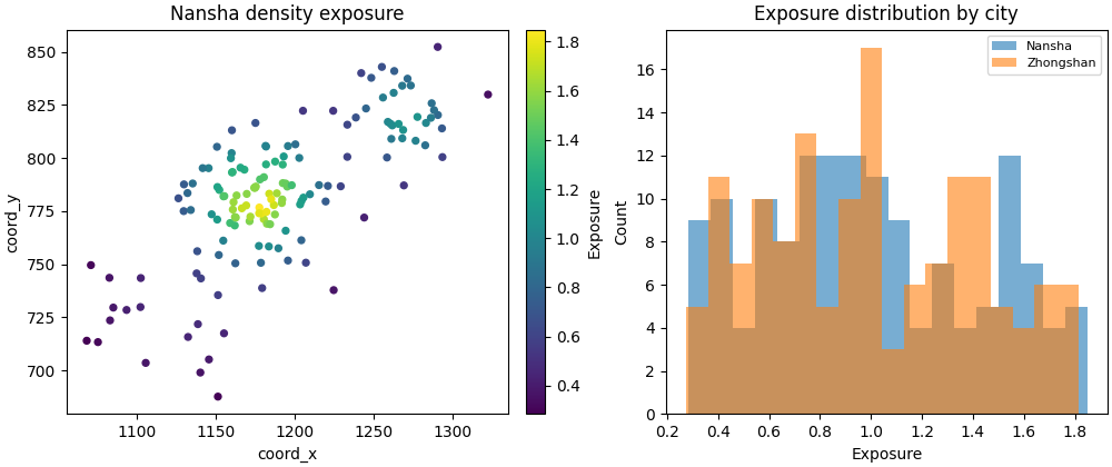
Build one compact visual preview

This preview is not part of the production builder itself. It is a teaching aid for the gallery page.

Left:

Nansha point map colored by exposure.

Right:

city-wise exposure histograms.

fig, axes = plt.subplots(
    1,
    2,
    figsize=(10.0, 4.2),
    constrained_layout=True,
)

# Point map for Nansha
ax = axes[0]
sub = expo_plot.loc[expo_plot["city"] == "Nansha"].copy()
sc = ax.scatter(
    sub["coord_x"].to_numpy(float),
    sub["coord_y"].to_numpy(float),
    c=sub["exposure"].to_numpy(float),
    s=18,
)
ax.set_title("Nansha density exposure")
ax.set_xlabel("coord_x")
ax.set_ylabel("coord_y")
fig.colorbar(sc, ax=ax, fraction=0.046, pad=0.04).set_label(
    "Exposure"
)

# Histograms
ax = axes[1]
for city in ["Nansha", "Zhongshan"]:
    sub = expo.loc[expo["city"] == city, "exposure"].to_numpy(float)
    ax.hist(sub, bins=18, alpha=0.6, label=city)
ax.set_title("Exposure distribution by city")
ax.set_xlabel("Exposure")
ax.set_ylabel("Count")
ax.legend(fontsize=8)

<matplotlib.legend.Legend object at 0x749e56e7db50>

Compare with uniform mode

The command also supports a pure uniform mode. That mode is useful when you want a placeholder exposure layer without introducing any density effect.

uniform_csv = tmp_dir / "exposure_uniform_gallery.csv"

make_exposure_main(
    [
         "--cities", "ns",
        "--ns-eval",
        str(ns_eval_csv),
        "--ns-future",
        str(ns_future_csv),
        "--mode",
        "uniform",
        "--out",
        str(uniform_csv),
    ],
    prog="make-exposure",
)

uniform_df = pd.read_csv(uniform_csv)

print("")
print("Uniform exposure preview")
print(uniform_df.head(8).to_string(index=False))

[OK] wrote /tmp/gp_sg_exposure_mzxsjmwk/exposure_uniform_gallery.csv

Uniform exposure preview
  city  sample_idx  exposure
Nansha           0    1.0000
Nansha           1    1.0000
Nansha           2    1.0000
Nansha           3    1.0000
Nansha           4    1.0000
Nansha           5    1.0000
Nansha           6    1.0000
Nansha           7    1.0000

Learn how to read this artifact

The output is intentionally minimal.

Each row contains:

• city

• sample_idx

• exposure

That means the artifact is designed to be joined back onto another table by (city, sample_idx) rather than to stand alone as a full spatial dataset.

What density exposure means here

In density mode, the script computes a simple geometric proxy:

• find the k nearest neighbors,

• compute the mean neighbor distance,

• take its inverse,

• normalize the resulting scores to mean 1.

So larger values indicate samples in denser local point regions, not necessarily regions with higher true population or damage.

Why deduplication matters

The builder concatenates eval and future point sets, then drops duplicate sample_idx values per city before computing exposure.

That is important because the same spatial sample often appears in both files, and we want one exposure value per logical sample, not one per file row.

Why this page belongs after make_district_grid.py

A useful support-layer workflow is:

1. build a boundary,

2. build a district grid,

3. build an exposure proxy,

4. then use those layers in cluster or hotspot summaries.

The artifacts are different, but they all reuse the same underlying point geometry.

Command-line version

The same lesson can be reproduced from the CLI.

Legacy dispatcher:

python -m scripts make-exposure \
  --ns-eval results/nansha_eval.csv \
  --ns-future results/nansha_future.csv \
  --zh-eval results/zhongshan_eval.csv \
  --zh-future results/zhongshan_future.csv \
  --mode density \
  --k 30 \
  --out exposure

Uniform mode:

python -m scripts make-exposure \
  --ns-src results/nansha_run \
  --split auto \
  --mode uniform \
  --out exposure_uniform

Modern CLI:

geoprior build exposure \
  --ns-src results/nansha_run \
  --zh-src results/zhongshan_run \
  --split auto \
  --mode density \
  --k 30 \
  --out exposure

The gallery page teaches the builder. The command line reproduces it in a workflow.