When cross-city reuse is useful, and when it is not

This application turns transferability into a deployment question rather than a benchmarking side note.

The practical question is simple:

Can a model trained in one city be reused in another city without losing the things that matter most for action?

For GeoPrior, the answer is intentionally nuanced. Cross-city reuse matters because a new city rarely starts with a fully mature training archive, a complete physical characterization, and enough time for a full model rebuild. A reusable model can shorten rollout. But rollout only matters if the transferred model still preserves:

1. useful deterministic skill,

2. calibrated uncertainty,

3. reliable threshold-risk information, and

4. stable hotspot prioritization.

Why this matters

A transfer model can look respectable on one error metric and still fail operationally. This happens when direct transfer keeps some broad spatial structure but distorts scale, coverage, or threshold probabilities. In that setting, the map may still look plausible while the ranking of action-first zones becomes unreliable.

This page therefore reads transferability as a staged audit:

• overall retention asks whether broad skill survives,

• horizon retention asks whether the degradation appears immediately or only at longer lead times,

• coverage–sharpness asks whether uncertainty remains decision-ready,

• risk skill asks whether exceedance probabilities remain trustworthy, and

• hotspot stability asks whether intervention priorities survive domain shift.

The compact tables below are reference-style values chosen to teach the reported pattern clearly: direct transfer degrades, while warm-start adaptation recovers much of the useful structure. When real xfer_results.csv and xfer_results.json files are available, the production workflow at the end of the page should replace these illustrative tables.

import numpy as np
import pandas as pd
import matplotlib.pyplot as plt

TARGET_COVERAGE = 0.80
RISK_THRESHOLD = 50.0
HOTSPOT_K = 100

CITY_COLORS = {
    "Nansha": "#1f77b4",
    "Zhongshan": "#e41a1c",
}

STRATEGY_LABELS = {
    "baseline": "target baseline",
    "transfer": "direct transfer",
    "warm": "warm-start",
}

STRATEGY_MARKERS = {
    "baseline": "o",
    "transfer": "^",
    "warm": "s",
}

STRATEGY_LINESTYLES = {
    "baseline": "-",
    "transfer": "--",
    "warm": "-",
}

STRATEGY_HATCH = {
    "baseline": "",
    "transfer": "//",
    "warm": "",
}


def build_transfer_table() -> pd.DataFrame:
    """Return a compact reference transfer audit table.

    The values are deliberately chosen to express the main
    transfer pattern in a readable way:

    - baseline defines the target-city reference,
    - direct transfer suffers a strong drop,
    - warm-start recovers much of the lost skill,
    - the Zhongshan → Nansha direction is harder.
    """
    rows = [
        {
            "direction": "Nansha → Zhongshan",
            "target_city": "Zhongshan",
            "strategy": "baseline",
            "r2_retention": 1.00,
            "mae_retention": 1.00,
            "coverage80": 0.81,
            "sharpness80_mm": 10.0,
            "brier": 0.071,
            "jaccard100": 1.00,
            "spearman100": 1.00,
        },
        {
            "direction": "Nansha → Zhongshan",
            "target_city": "Zhongshan",
            "strategy": "transfer",
            "r2_retention": 0.32,
            "mae_retention": 0.44,
            "coverage80": 0.56,
            "sharpness80_mm": 15.3,
            "brier": 0.183,
            "jaccard100": 0.34,
            "spearman100": 0.39,
        },
        {
            "direction": "Nansha → Zhongshan",
            "target_city": "Zhongshan",
            "strategy": "warm",
            "r2_retention": 0.83,
            "mae_retention": 0.90,
            "coverage80": 0.79,
            "sharpness80_mm": 11.8,
            "brier": 0.093,
            "jaccard100": 0.67,
            "spearman100": 0.74,
        },
        {
            "direction": "Zhongshan → Nansha",
            "target_city": "Nansha",
            "strategy": "baseline",
            "r2_retention": 1.00,
            "mae_retention": 1.00,
            "coverage80": 0.86,
            "sharpness80_mm": 33.1,
            "brier": 0.084,
            "jaccard100": 1.00,
            "spearman100": 1.00,
        },
        {
            "direction": "Zhongshan → Nansha",
            "target_city": "Nansha",
            "strategy": "transfer",
            "r2_retention": 0.18,
            "mae_retention": 0.31,
            "coverage80": 0.49,
            "sharpness80_mm": 25.4,
            "brier": 0.224,
            "jaccard100": 0.24,
            "spearman100": 0.29,
        },
        {
            "direction": "Zhongshan → Nansha",
            "target_city": "Nansha",
            "strategy": "warm",
            "r2_retention": 0.76,
            "mae_retention": 0.84,
            "coverage80": 0.78,
            "sharpness80_mm": 35.5,
            "brier": 0.117,
            "jaccard100": 0.58,
            "spearman100": 0.65,
        },
    ]
    return pd.DataFrame(rows)


def build_horizon_retention() -> pd.DataFrame:
    """Return horizon-wise RMSE retention.

    Retention is defined on a higher-is-better scale, where
    1.0 means parity with the target-city baseline.
    """
    rows = [
        {
            "direction": "Nansha → Zhongshan",
            "strategy": "baseline",
            "H1": 1.00,
            "H2": 1.00,
            "H3": 1.00,
        },
        {
            "direction": "Nansha → Zhongshan",
            "strategy": "transfer",
            "H1": 0.46,
            "H2": 0.39,
            "H3": 0.34,
        },
        {
            "direction": "Nansha → Zhongshan",
            "strategy": "warm",
            "H1": 0.90,
            "H2": 0.84,
            "H3": 0.80,
        },
        {
            "direction": "Zhongshan → Nansha",
            "strategy": "baseline",
            "H1": 1.00,
            "H2": 1.00,
            "H3": 1.00,
        },
        {
            "direction": "Zhongshan → Nansha",
            "strategy": "transfer",
            "H1": 0.34,
            "H2": 0.29,
            "H3": 0.26,
        },
        {
            "direction": "Zhongshan → Nansha",
            "strategy": "warm",
            "H1": 0.85,
            "H2": 0.78,
            "H3": 0.74,
        },
    ]
    return pd.DataFrame(rows)


def build_reliability_curves() -> pd.DataFrame:
    """Return reference reliability curves.

    These points are intentionally simple.  They show the main
    transfer lesson without pretending to be a hidden source
    table.
    """
    bins = np.array([0.05, 0.15, 0.25, 0.40, 0.55, 0.70, 0.85])

    defs = [
        (
            "Nansha → Zhongshan",
            "baseline",
            np.array([0.04, 0.13, 0.24, 0.39, 0.54, 0.70, 0.84]),
        ),
        (
            "Nansha → Zhongshan",
            "transfer",
            np.array([0.09, 0.21, 0.31, 0.40, 0.48, 0.56, 0.61]),
        ),
        (
            "Nansha → Zhongshan",
            "warm",
            np.array([0.05, 0.15, 0.25, 0.39, 0.53, 0.68, 0.80]),
        ),
        (
            "Zhongshan → Nansha",
            "baseline",
            np.array([0.06, 0.16, 0.26, 0.41, 0.56, 0.72, 0.87]),
        ),
        (
            "Zhongshan → Nansha",
            "transfer",
            np.array([0.12, 0.24, 0.37, 0.46, 0.52, 0.58, 0.63]),
        ),
        (
            "Zhongshan → Nansha",
            "warm",
            np.array([0.07, 0.17, 0.27, 0.42, 0.55, 0.69, 0.81]),
        ),
    ]

    rows = []
    for direction, strategy, obs in defs:
        for p, y in zip(bins, obs):
            rows.append(
                {
                    "direction": direction,
                    "strategy": strategy,
                    "predicted": p,
                    "observed": y,
                }
            )
    return pd.DataFrame(rows)


def build_transfer_summary(
    overall: pd.DataFrame,
) -> pd.DataFrame:
    """Add application-friendly interpretation tags."""
    out = overall.copy()

    out["coverage_gap"] = np.abs(
        out["coverage80"] - TARGET_COVERAGE
    )
    out["risk_penalty_vs_baseline"] = out.groupby("direction")[
        "brier"
    ].transform(lambda s: s - s.iloc[0])

    def _status(row: pd.Series) -> str:
        if row["strategy"] == "baseline":
            return "reference"
        if (
            row["r2_retention"] >= 0.75
            and row["coverage_gap"] <= 0.03
            and row["jaccard100"] >= 0.55
        ):
            return "deployable after adaptation"
        if row["jaccard100"] >= 0.30:
            return "screening only"
        return "not ready"

    out["deployment_status"] = out.apply(_status, axis=1)
    return out


def make_rollout_cards() -> list[dict[str, str]]:
    """Return short rollout recommendations."""
    return [
        {
            "title": "Zero-shot transfer",
            "body": (
                "Useful for exploratory screening and quick visual "
                "comparison, but not strong enough for calibrated "
                "deployment or final hotspot ranking."
            ),
        },
        {
            "title": "Warm-start adaptation",
            "body": (
                "The best compromise when a new city has modest "
                "local data.  It preserves the transferable spatial "
                "organisation while restoring scale and probability."
            ),
        },
        {
            "title": "Target baseline",
            "body": (
                "The reference ceiling for that city.  It remains the "
                "right comparator whenever transferability is claimed."
            ),
        },
    ]

Reference audit tables

The tables below establish the reading order.

• r2_retention and mae_retention tell us how much deterministic skill survives after transfer.

• coverage80 and sharpness80_mm show whether the intervals remain useful rather than merely wide.

• brier tests threshold-risk quality for the event abs(s) >= 50 mm/yr.

• jaccard100 and spearman100 ask the planning question directly: do the same top-100 zones remain near the top of the action list?

overall = build_transfer_table()
horizon = build_horizon_retention()
reliability = build_reliability_curves()
summary = build_transfer_summary(overall)

print("Reference transfer audit:\n")
print(overall.round(3).to_string(index=False))

print("\nDeployment-oriented summary:\n")
print(
    summary[
        [
            "direction",
            "strategy",
            "coverage_gap",
            "risk_penalty_vs_baseline",
            "deployment_status",
        ]
    ]
    .round(3)
    .to_string(index=False)
)

Reference transfer audit:

         direction target_city strategy  r2_retention  mae_retention  coverage80  sharpness80_mm  brier  jaccard100  spearman100
Nansha → Zhongshan   Zhongshan baseline          1.00           1.00        0.81            10.0  0.071        1.00         1.00
Nansha → Zhongshan   Zhongshan transfer          0.32           0.44        0.56            15.3  0.183        0.34         0.39
Nansha → Zhongshan   Zhongshan     warm          0.83           0.90        0.79            11.8  0.093        0.67         0.74
Zhongshan → Nansha      Nansha baseline          1.00           1.00        0.86            33.1  0.084        1.00         1.00
Zhongshan → Nansha      Nansha transfer          0.18           0.31        0.49            25.4  0.224        0.24         0.29
Zhongshan → Nansha      Nansha     warm          0.76           0.84        0.78            35.5  0.117        0.58         0.65

Deployment-oriented summary:

         direction strategy  coverage_gap  risk_penalty_vs_baseline           deployment_status
Nansha → Zhongshan baseline          0.01                     0.000                   reference
Nansha → Zhongshan transfer          0.24                     0.112              screening only
Nansha → Zhongshan     warm          0.01                     0.022 deployable after adaptation
Zhongshan → Nansha baseline          0.06                     0.000                   reference
Zhongshan → Nansha transfer          0.31                     0.140                   not ready
Zhongshan → Nansha     warm          0.02                     0.033 deployable after adaptation

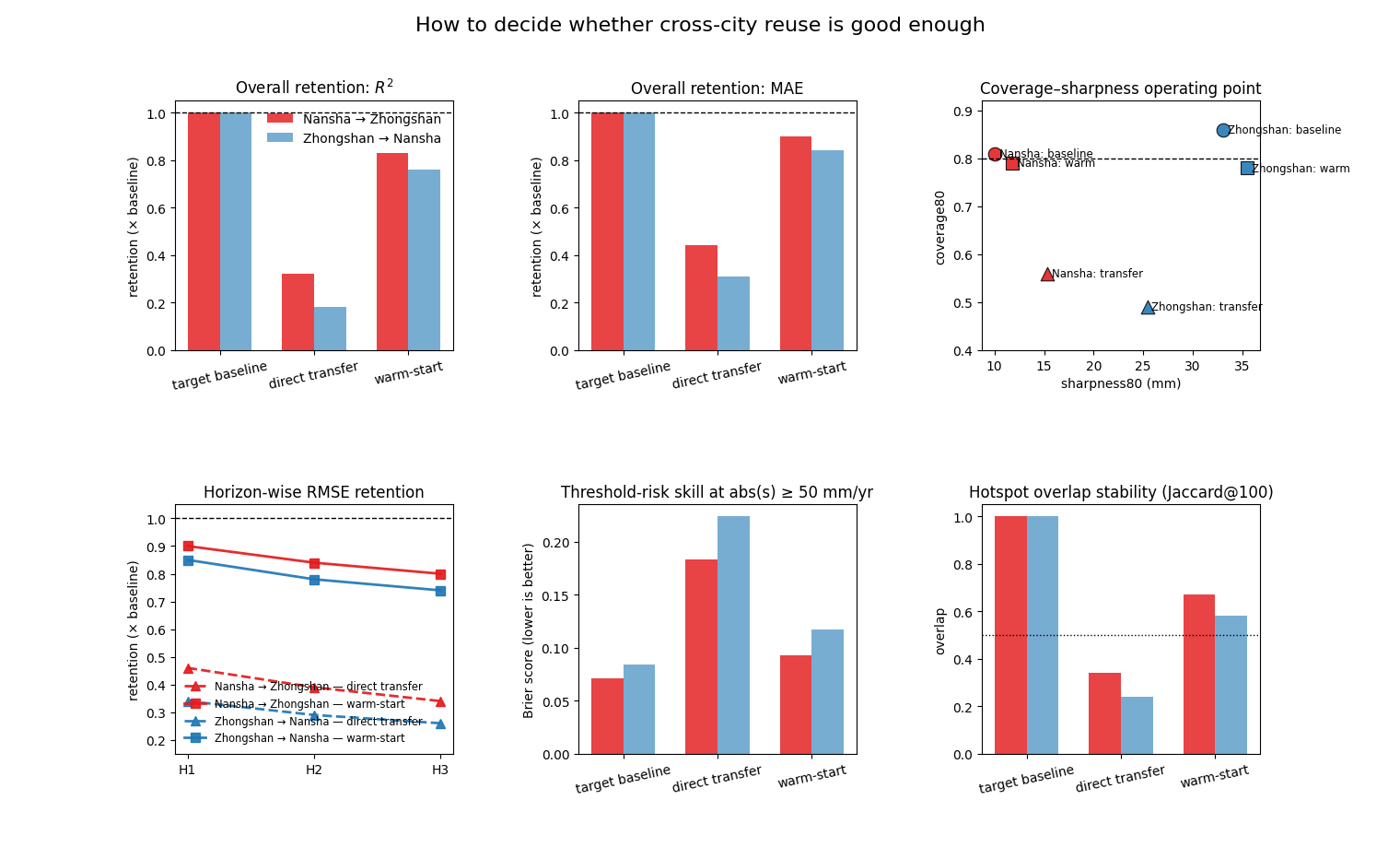
Transfer dashboard — retention, uncertainty, and risk

This dashboard follows the same logic as the production transfer scripts:

1. overall retention relative to the target-city baseline,

2. horizon retention to see whether the drop appears early,

3. coverage–sharpness operating point, and

4. threshold-risk skill.

The message to watch for is not simply “transfer is worse”. The deeper message is how it is worse. Direct transfer loses both scale and calibration, while warm-start restores much of the useful structure.

fig = plt.figure(figsize=(15.2, 9.2))
grid = fig.add_gridspec(2, 3, wspace=0.45, hspace=0.62)

ax_a = fig.add_subplot(grid[0, 0])
ax_b = fig.add_subplot(grid[0, 1])
ax_c = fig.add_subplot(grid[0, 2])
ax_d = fig.add_subplot(grid[1, 0])
ax_e = fig.add_subplot(grid[1, 1])
ax_f = fig.add_subplot(grid[1, 2])

bar_strats = ["baseline", "transfer", "warm"]
directions = [
    "Nansha → Zhongshan",
    "Zhongshan → Nansha",
]

x = np.arange(len(bar_strats))
width = 0.34

for i, direction in enumerate(directions):
    sub = overall[overall["direction"] == direction].set_index(
        "strategy"
    )
    vals = [sub.loc[s, "r2_retention"] for s in bar_strats]
    ax_a.bar(
        x + (i - 0.5) * width,
        vals,
        width=width,
        color=CITY_COLORS[sub.iloc[0]["target_city"]],
        alpha=0.82 if i == 0 else 0.60,
        label=direction,
    )

ax_a.axhline(1.0, color="black", linestyle="--", linewidth=1.0)
ax_a.set_title("Overall retention: $R^2$")
ax_a.set_ylabel("retention (× baseline)")
ax_a.set_xticks(x, [STRATEGY_LABELS[s] for s in bar_strats], rotation=12)
ax_a.legend(frameon=False, loc="upper right")

for i, direction in enumerate(directions):
    sub = overall[overall["direction"] == direction].set_index(
        "strategy"
    )
    vals = [sub.loc[s, "mae_retention"] for s in bar_strats]
    ax_b.bar(
        x + (i - 0.5) * width,
        vals,
        width=width,
        color=CITY_COLORS[sub.iloc[0]["target_city"]],
        alpha=0.82 if i == 0 else 0.60,
    )

ax_b.axhline(1.0, color="black", linestyle="--", linewidth=1.0)
ax_b.set_title("Overall retention: MAE")
ax_b.set_ylabel("retention (× baseline)")
ax_b.set_xticks(x, [STRATEGY_LABELS[s] for s in bar_strats], rotation=12)

for direction in directions:
    sub = overall[overall["direction"] == direction]
    color = CITY_COLORS[sub.iloc[0]["target_city"]]
    for _, row in sub.iterrows():
        ax_c.scatter(
            row["sharpness80_mm"],
            row["coverage80"],
            s=110,
            color=color,
            marker=STRATEGY_MARKERS[row["strategy"]],
            edgecolor="black",
            linewidth=0.8,
            alpha=0.88,
        )
        ax_c.text(
            row["sharpness80_mm"] + 0.45,
            row["coverage80"],
            f"{direction.split()[0]}: {row['strategy']}",
            fontsize=8.5,
            va="center",
        )

ax_c.axhline(
    TARGET_COVERAGE,
    color="black",
    linestyle="--",
    linewidth=1.0,
)
ax_c.set_title("Coverage–sharpness operating point")
ax_c.set_xlabel("sharpness80 (mm)")
ax_c.set_ylabel("coverage80")
ax_c.set_ylim(0.40, 0.92)

horizons = ["H1", "H2", "H3"]
for direction in directions:
    sub = horizon[horizon["direction"] == direction].set_index(
        "strategy"
    )
    color = CITY_COLORS[
        overall[overall["direction"] == direction]
        .iloc[0]["target_city"]
    ]
    for strategy in ["transfer", "warm"]:
        vals = [sub.loc[strategy, h] for h in horizons]
        ax_d.plot(
            horizons,
            vals,
            color=color,
            linestyle=STRATEGY_LINESTYLES[strategy],
            marker=STRATEGY_MARKERS[strategy],
            linewidth=2.0,
            markersize=7,
            alpha=0.92,
            label=f"{direction} — {STRATEGY_LABELS[strategy]}",
        )

ax_d.axhline(1.0, color="black", linestyle="--", linewidth=1.0)
ax_d.set_title("Horizon-wise RMSE retention")
ax_d.set_ylabel("retention (× baseline)")
ax_d.set_ylim(0.15, 1.05)
ax_d.legend(frameon=False, loc="lower left", fontsize=8.3)

for i, direction in enumerate(directions):
    sub = overall[overall["direction"] == direction].set_index(
        "strategy"
    )
    vals = [sub.loc[s, "brier"] for s in bar_strats]
    ax_e.bar(
        x + (i - 0.5) * width,
        vals,
        width=width,
        color=CITY_COLORS[sub.iloc[0]["target_city"]],
        alpha=0.82 if i == 0 else 0.60,
    )

ax_e.set_title(
    f"Threshold-risk skill at abs(s) ≥ {RISK_THRESHOLD:.0f} mm/yr"
)
ax_e.set_ylabel("Brier score (lower is better)")
ax_e.set_xticks(x, [STRATEGY_LABELS[s] for s in bar_strats], rotation=12)

for i, direction in enumerate(directions):
    sub = overall[overall["direction"] == direction].set_index(
        "strategy"
    )
    vals = [sub.loc[s, "jaccard100"] for s in bar_strats]
    ax_f.bar(
        x + (i - 0.5) * width,
        vals,
        width=width,
        color=CITY_COLORS[sub.iloc[0]["target_city"]],
        alpha=0.82 if i == 0 else 0.60,
    )

ax_f.axhline(0.50, color="black", linestyle=":", linewidth=1.0)
ax_f.set_title(f"Hotspot overlap stability (Jaccard@{HOTSPOT_K})")
ax_f.set_ylabel("overlap")
ax_f.set_xticks(x, [STRATEGY_LABELS[s] for s in bar_strats], rotation=12)
ax_f.set_ylim(0.0, 1.05)

fig.suptitle(
    "How to decide whether cross-city reuse is good enough",
    y=0.98,
    fontsize=16,
)

Text(0.5, 0.98, 'How to decide whether cross-city reuse is good enough')

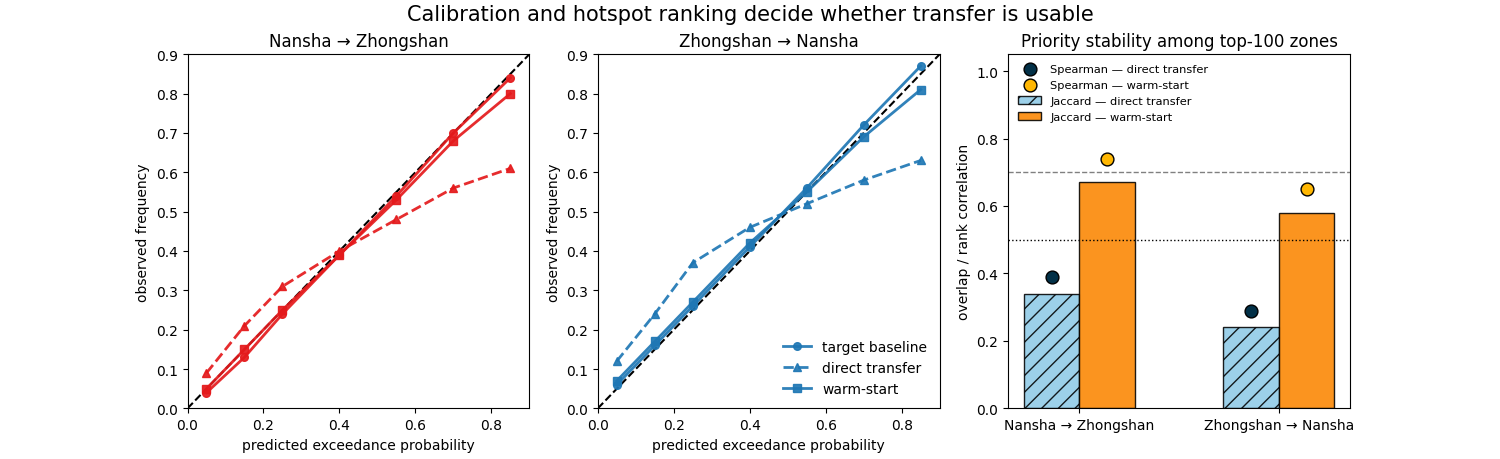
Reliability view and hotspot rank stability

The previous dashboard already shows that warm-start is closer to the target baseline. This second view explains why that matters operationally.

A transfer model can still resemble the target city in a broad visual sense while assigning the wrong exceedance probabilities or shuffling the top-priority zones. That is why reliability and hotspot stability deserve their own readout.

fig, axes = plt.subplots(1, 3, figsize=(15.0, 4.6))
ax_a, ax_b, ax_c = axes

for ax, direction in zip(axes[:2], directions):
    ax.plot([0.0, 1.0], [0.0, 1.0], color="black", linestyle="--")
    sub = reliability[reliability["direction"] == direction]
    target_city = overall[
        overall["direction"] == direction
    ].iloc[0]["target_city"]
    color = CITY_COLORS[target_city]

    for strategy in ["baseline", "transfer", "warm"]:
        cur = sub[sub["strategy"] == strategy]
        ax.plot(
            cur["predicted"],
            cur["observed"],
            color=color,
            linestyle=STRATEGY_LINESTYLES[strategy],
            marker=STRATEGY_MARKERS[strategy],
            linewidth=2.0,
            markersize=5.5,
            label=STRATEGY_LABELS[strategy],
            alpha=0.92,
        )

    ax.set_xlim(0.0, 0.90)
    ax.set_ylim(0.0, 0.90)
    ax.set_title(direction)
    ax.set_xlabel("predicted exceedance probability")
    ax.set_ylabel("observed frequency")

ax_b.legend(frameon=False, loc="lower right")

plot_rows = []
for direction in directions:
    cur = overall[
        (overall["direction"] == direction)
        & (overall["strategy"].isin(["transfer", "warm"]))
    ].copy()
    plot_rows.append(cur)
plot_rows = pd.concat(plot_rows, ignore_index=True)

x0 = np.arange(len(directions))
width = 0.28
for j, strategy in enumerate(["transfer", "warm"]):
    sub = plot_rows[plot_rows["strategy"] == strategy]
    ax_c.bar(
        x0 + (j - 0.5) * width,
        sub["jaccard100"],
        width=width,
        color="#8ecae6" if strategy == "transfer" else "#fb8500",
        edgecolor="black",
        hatch=STRATEGY_HATCH[strategy],
        alpha=0.88,
        label=f"Jaccard — {STRATEGY_LABELS[strategy]}",
    )
    ax_c.scatter(
        x0 + (j - 0.5) * width,
        sub["spearman100"],
        s=85,
        color="#023047" if strategy == "transfer" else "#ffb703",
        edgecolor="black",
        zorder=3,
        label=f"Spearman — {STRATEGY_LABELS[strategy]}",
    )

ax_c.axhline(0.50, color="black", linestyle=":", linewidth=1.0)
ax_c.axhline(0.70, color="gray", linestyle="--", linewidth=1.0)
ax_c.set_xticks(x0, directions)
ax_c.set_ylim(0.0, 1.05)
ax_c.set_title(f"Priority stability among top-{HOTSPOT_K} zones")
ax_c.set_ylabel("overlap / rank correlation")
ax_c.legend(frameon=False, loc="upper left", fontsize=8.2)

fig.suptitle(
    "Calibration and hotspot ranking decide whether transfer is usable",
    y=0.99,
    fontsize=15,
)

Text(0.5, 0.99, 'Calibration and hotspot ranking decide whether transfer is usable')

Reading protocol

The transfer audit should end with a rollout rule rather than with another decorative figure. The table below turns the main findings into a practical approval protocol for new cities.

Transfer rollout protocol

Rule	Reading guidance	Rollout implication
Direct transfer is a screening test	Direct transfer is usually not rejected because the map becomes meaningless. It is rejected because uncertainty, calibration, and threshold probabilities are no longer strong enough for decision support.	Use zero-shot transfer as a rapid screening layer or as a stress test of retained structure, not as a final operational product unless the forecast and risk audits remain acceptable.
Warm-start adaptation can already be enough	Warm-start adaptation does not need to recover full parity with the target-city baseline to be useful. It only needs to restore enough deterministic skill, calibration quality, and hotspot stability that the action list remains credible.	Approve warm-start rollout when the model recovers usable forecast behavior and a defensible prioritization signal, even if some gap to the target baseline remains.
Transfer preserves structure more easily than amplitude	The most transferable part of the model is often the broader spatial and temporal organization, not the absolute amplitude. That is why direct transfer may keep some visual resemblance while still failing the risk and prioritization tests.	Treat retained pattern structure as encouraging, but do not confuse visual similarity with deployment readiness. Approval should depend on both forecast quality and action-list reliability.

Note

Operational takeaway: transfer should be approved only after the model passes both a forecast audit and a prioritization audit.

Practical reading

The main conclusion of this application is not that transfer either “works” or “fails” in a binary sense. The more informative result is that the transfer regime itself matters.

Direct zero-shot reuse is useful as a stress test because it shows what survives a basin-scale shift without local adaptation. In that regime, broad structural signal can remain visible, but calibration, retained point skill, and downstream prioritization quality may no longer be strong enough for confident deployment.

Warm-start adaptation changes the interpretation. It does not simply improve a few aggregate metrics; it restores a more usable balance between retained predictive skill, uncertainty quality, and hotspot-level consistency. That is the practical meaning of transferability in GeoPrior: not blind portability, but the ability to recover scientifically useful structure with modest local adaptation.

This distinction is important for deployment. A cross-city model may still be informative when used as a screening layer, an initialization point, or a rapid-response prior, even if it is not yet acceptable as a final city-specific forecasting system. The transfer audit therefore helps separate three operational roles:

• screening without retraining,

• warm-start adaptation for fast local recovery,

• full retraining when the shift is too large.

In that sense, this page should be read less as a generic model comparison and more as a deployment decision study. It asks not only whether knowledge transfers, but which parts of that knowledge remain decision-relevant after the shift and what level of adaptation is needed before the forecasts become trustworthy again.

That reading is also consistent with the broader scientific message: zero-shot reuse degrades under basin-scale distribution shift, whereas warm-start adaptation recovers more usable skill and more stable hotspot signals, making transfer a structured pathway to rollout rather than a shortcut around local validation.

plt.show()

From case study to real artifacts

The miniature case study above is self-contained, which is ideal for a gallery page. In production, the same transfer audit should be driven by the existing transfer backends so that the performance views, the uncertainty views, and the risk-transfer views remain aligned on the same xfer_results package.

geoprior plot transfer \
  --src results/xfer/nansha__zhongshan \
  --split val \
  --strategies baseline xfer warm \
  --calib-modes none source target \
  --metric-top mae \
  --metric-bottom r2 \
  --out transfer_overview.png

geoprior plot transfer-impact \
  --src results/xfer/nansha__zhongshan \
  --split val \
  --calib source \
  --threshold 50 \
  --add-hotspots true \
  --hotspot-k 100 \
  --hotspot-score q50 \
  --hotspot-horizon H3 \
  --hotspot-style bar \
  --out transfer_impact.png

geoprior plot xfer-transferability \
  --src results/xfer/nansha__zhongshan \
  --split val \
  --strategies baseline xfer warm \
  --calib-modes none source target \
  --metric-top mae \
  --metric-bottom mse \
  --out transferability_grid.png

from geoprior.scripts.plot_transfer import (
    figSx_xfer_transferability_main,
)
from geoprior.scripts.plot_xfer_impact import (
    figSx_xfer_impact_main,
)

figSx_xfer_transferability_main(
    [
        "--src", "results/xfer/nansha__zhongshan",
        "--split", "val",
        "--strategies", "baseline", "xfer", "warm",
        "--calib-modes", "none", "source", "target",
        "--metric-top", "mae",
        "--metric-bottom", "r2",
        "--out", "transfer_overview.png",
    ]
)

figSx_xfer_impact_main(
    [
        "--src", "results/xfer/nansha__zhongshan",
        "--split", "val",
        "--calib", "source",
        "--threshold", "50",
        "--add-hotspots", "true",
        "--hotspot-k", "100",
        "--hotspot-score", "q50",
        "--hotspot-horizon", "H3",
        "--hotspot-style", "bar",
        "--out", "transfer_impact.png",
    ]
)

A good scientific reading order is:

1. overall retention and horizon behavior,

2. coverage, sharpness, and reliability,

3. threshold-risk skill and hotspot stability,

4. final rollout judgment: screening only, warm-start, or retrain.

That production sequence is what turns the gallery lesson into a real deployment audit for new city pairs, updated transfer runs, or revised adaptation strategies.