
Figure generation#
This gallery focuses on paper-ready and analysis-ready plotting workflows in GeoPrior.
Unlike the examples in tables_and_summaries/, the pages collected
here begin from plotting scripts whose main purpose is to generate
visual outputs: main figures, supplementary figures, diagnostic panels,
sensitivity plots, transfer figures, and spatial analytics views.
The emphasis is therefore on communication through figures. These examples show how GeoPrior turns model outputs, diagnostic signals, and support artifacts into interpretable visual summaries that can be used for analysis, reporting, and manuscript preparation.
Typical outputs in this section include:
publication-style PNG, SVG, or EPS figures,
multi-panel diagnostic layouts,
sensitivity heatmaps and comparison plots,
spatial forecast maps and hotspot analytics panels,
transferability and impact figures,
validation and cumulative-summary plots.
In other words, this gallery is about building the figures that communicate results, not the intermediate artifacts that those figures depend on.
What this gallery teaches#
Most pages in this section follow the same broad pattern:
create or load a compact synthetic input,
call the real GeoPrior plotting script,
inspect the generated figure files,
explain how to read and interpret the main panels.
Even when a page prints small tables or intermediate values, the main goal remains the same: to explain the figure and its interpretation.
Module guide#
Module |
Main output |
Purpose |
|---|---|---|
|
Relationship figure |
Plot driver-response relationships to show how key forcing or context variables relate to predicted behavior. |
|
Ablation comparison figure |
Plot the core ablation comparisons used to interpret the main model-design trade-offs. |
|
Uncertainty figure |
Plot the main uncertainty diagnostics, including calibration and reliability-oriented views. |
|
Spatial forecast maps |
Plot the main spatial forecast maps and multi-panel forecast layouts. |
|
Physics sanity figure |
Plot sanity checks for the physics-informed components. |
|
Physics map panels |
Plot map-based views of learned or inferred physics quantities. |
|
Field diagnostic figure |
Plot field-level diagnostics for physical parameters and related outputs. |
|
Profile diagnostics |
Plot profile-style physics diagnostics, typically for appendix or supplementary interpretation. |
|
Parity / agreement figure |
Plot lithology-related parity or agreement diagnostics. |
|
Sensitivity surface figure |
Plot sensitivity surfaces and ablation-response summaries. |
|
Physics sensitivity figure |
Plot the response of physical metrics or residuals to sensitivity settings. |
|
Identifiability figure |
Plot SM3 identifiability diagnostics. |
|
Bounds / ridge summary |
Plot ridge and bounds summaries for SM3-style identifiability experiments. |
|
Log-offset diagnostics |
Plot SM3 log-offset diagnostics and related parameter-behavior summaries. |
|
Transferability figure |
Plot transferability performance across source-target settings. |
|
Transfer impact figure |
Plot transfer impact in terms of retention, hotspot overlap, and related measures. |
|
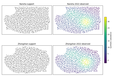
Validation figure |
Plot external point-support validation results. |
|
Cumulative summary figure |
Plot cumulative geo-style summaries across years or scenarios. |
|
Hotspot analytics figure |
Plot hotspot analytics views that summarize spatial hotspot behavior over time or across settings. |
|
Supplementary uncertainty panels |
Plot additional uncertainty panels beyond the main uncertainty figure. |
Reading path#
A useful way to move through this gallery is to follow the logic of a complete visual analysis workflow:
begin with core model-behavior figures,
continue to uncertainty and sensitivity structure,
move into spatial and physics-aware visual diagnostics,
finish with transfer, impact, and validation views.
That is why the examples are grouped by plotting purpose rather than only by command family.
Gallery organization#
Core result figures#
These examples correspond most directly to the central narrative figures of the GeoPrior workflow. They are often the best place to start when you want a high-level visual understanding of model behavior and main results.
The main pages in this group are:
plot_driver_response.pyplot_core_ablation.pyplot_uncertainty.pyplot_spatial_forecasts.py
Physics and mechanistic diagnostics#
These examples focus on the physical structure of the model and on the interpretation of learned or inferred physics fields. They are most useful when you want to inspect whether the scientific behavior exposed by the model remains interpretable and internally coherent.
The main pages in this group are:
plot_physics_sanity.pyplot_physics_maps.pyplot_physics_fields.pyplot_physics_profiles.pyplot_litho_parity.py
Sensitivity and identifiability#
These examples focus on how results change under different weights, priors, constraints, or identifiability settings. They are particularly helpful when comparing training regimes or understanding the robustness of the formulation.
The main pages in this group are:
plot_ablations_sensitivity.pyplot_physics_sensitivity.pyplot_sm3_identifiability.pyplot_sm3_bounds_ridge_summary.pyplot_sm3_log_offsets.py
Transfer, impact, and validation#
These examples focus on cross-city transfer, downstream impact, and out-of-sample validation. They are especially useful when the goal is to understand generalization, downstream relevance, or practical forecast usefulness beyond a single training context.
The main pages in this group are:
plot_xfer_transferability.pyplot_xfer_impact.pyplot_external_validation.pyplot_geo_cumulative.pyplot_hotspot_analytics.py
Supplementary and extended visual analyses#
These examples provide additional visual depth beyond the core figure set and are useful when a workflow needs more detail than the main results pages alone provide.
The main page in this group is:
plot_uncertainty_extras.py
Why this separation matters#
This gallery deliberately keeps three concerns distinct:
artifact construction,
plot generation,
figure interpretation.
That separation makes the workflow easier to understand. It also helps users distinguish between commands that build reusable analysis products, scripts that turn those products into figures, and pages that focus on explaining what the resulting visuals actually mean.
Notes#
These examples are intentionally compact and lesson-oriented.
The scripts in this section are plot-first: they may print small summaries, but their main output is a figure file.
A useful rule of thumb is:
tables_and_summaries/builds reusable artifacts,model_inspection/explains helper-based diagnostics,figure_generation/turns results into visual outputs.
Many of these scripts are naturally suited to PNG, SVG, or EPS export for manuscripts, appendices, reports, and presentation material.
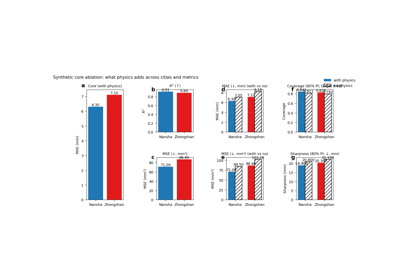
Core ablation: learning what physics adds to the workflow
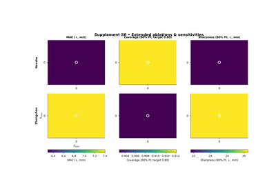
Ablations and sensitivities: learning where the model behaves well in lambda space
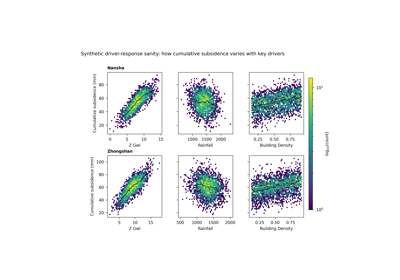
Driver-response plots: learning how the response moves with the drivers
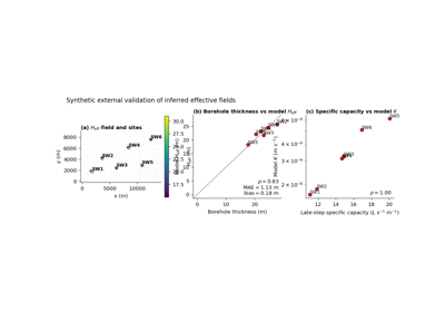
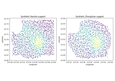
External validation: comparing inferred effective fields against independent site evidence
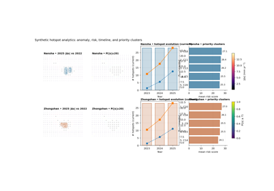
Hotspot analytics: turning future forecasts into decision-ready priority maps
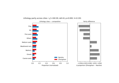
Lithology parity: comparing the geological composition of the two cities
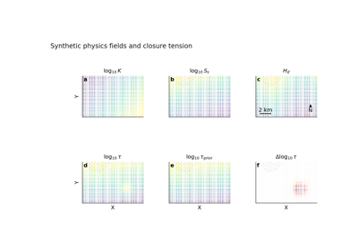
Physics fields: learning to read the physical story in a map
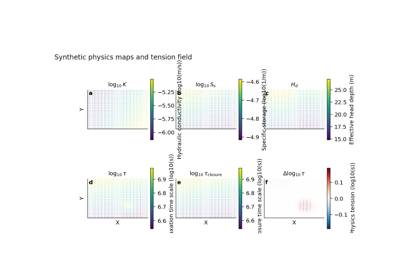
Physics maps: turning pointwise payloads into readable spatial fields
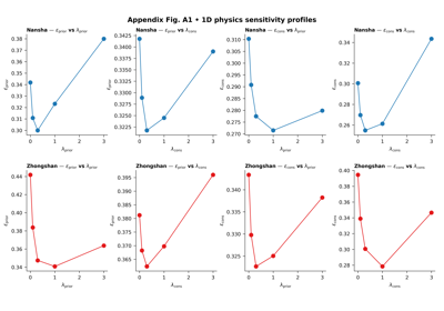
Physics profiles: reducing a 2D lambda landscape into readable 1D lessons
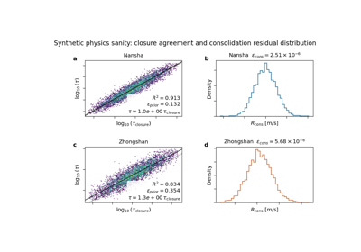
Physics sanity: checking closure agreement and residual behavior
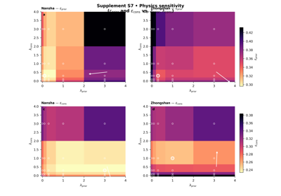
Physics sensitivity: learning how lambda choices reshape the physics diagnostics
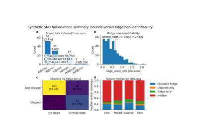
SM3 bounds versus ridge: learning the two main failure modes
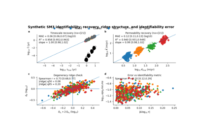
SM3 identifiability: learning when recovery is accurate and when parameters slide along a ridge
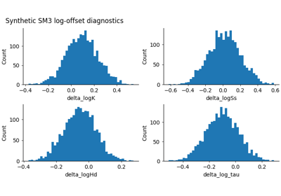
SM3 log offsets: learning where the inferred fields drift from their priors
Spatial forecasts: how to read observed maps, fitted maps, and future forecast maps together
Cross-city transferability: learning what survives transfer between cities
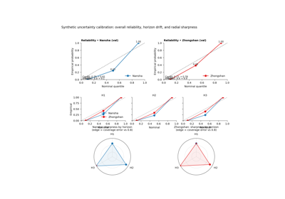
Forecast uncertainty: learning how calibration behaves across cities and horizons
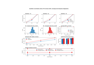
Expanded uncertainty diagnostics: learning what the main uncertainty figure still hides
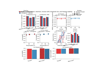
Transfer impact: what transfer changes for retention, risk, and hotspot stability
Cross-city transferability (v3.2): what survives when a workflow moves to the other city