
Note
Go to the end to download the full example code.
Assign boreholes to the nearest city cloud#
This example teaches how to use GeoPrior’s
assign-boreholes build utility.
Unlike the earlier builders in tables_and_summaries, this command
is not about sampling, clustering, or extracting one subset from a
single city table. Instead, it solves a very practical multi-city
integration task:
given one borehole or external-validation table, decide which city point cloud each borehole belongs to.
Why this matters#
Nearest-city assignment is useful when you need to:
separate one mixed validation file into per-city subsets,
route boreholes to the right Stage-1 processed footprint,
compare full-city validation metrics city by city,
inspect which boreholes sit close to the boundary between cities,
or prepare later command-line workflows that expect one file per city.
That is exactly what assign-boreholes is for.
What this lesson teaches#
We will:
build two realistic synthetic city clouds,
save them into Stage-1-like folders,
create one synthetic borehole validation table,
run the real
assign-boreholescommand,inspect the combined and per-city CSV outputs,
visualize the nearest-city assignment,
finish with direct command-line examples.
Imports#
We call the real production CLI entrypoint from the project code. For the synthetic city geometry, we reuse the shared spatial-support helpers instead of drawing arbitrary random points.
from __future__ import annotations

import tempfile
from pathlib import Path

import matplotlib.pyplot as plt
import numpy as np
import pandas as pd

from geoprior.cli.build_assign_boreholes import (
    build_assign_boreholes_main,
)
from geoprior.scripts import utils as script_utils
Step 1 - Build two synthetic city supports#
The command ultimately assigns boreholes against one or more city point clouds. To make the lesson realistic, we generate two compact projected supports that behave like two different Stage-1 cities.
The parameter comments are intentionally explicit so users can see how the synthetic geography is controlled.
Key parameters#
- city:
Human-readable city label stored in the support.
- center_x, center_y:
Center of the projected city footprint.
- span_x, span_y:
Half-width and half-height of the support extent in metres.
- nx, ny:
Mesh density before masking.
- jitter_x, jitter_y:
Small perturbations so the support is not a perfect grid.
- footprint:
Synthetic urban shape retained after masking.
- keep_frac:
Fraction of masked support points to keep.
- seed:
Keeps the support reproducible.
ns_support = script_utils.make_spatial_support(
    script_utils.SpatialSupportSpec(
        city="Nansha",
        center_x=12_500.0,
        center_y=8_200.0,
        span_x=3_400.0,
        span_y=2_500.0,
        nx=30,
        ny=22,
        jitter_x=36.0,
        jitter_y=32.0,
        footprint="nansha_like",
        keep_frac=0.90,
        seed=31,
    )
)

zh_support = script_utils.make_spatial_support(
    script_utils.SpatialSupportSpec(
        city="Zhongshan",
        center_x=24_800.0,
        center_y=9_400.0,
        span_x=3_800.0,
        span_y=2_800.0,
        nx=30,
        ny=22,
        jitter_x=40.0,
        jitter_y=34.0,
        footprint="zhongshan_like",
        keep_frac=0.90,
        seed=47,
    )
)
Step 2 - Create Stage-1-like processed city CSVs#
assign-boreholes can resolve city clouds from several input forms.
In this lesson, we use repeated --stage1-dir arguments because
that reflects a very natural workflow:
Stage-1 has already produced processed city tables,
we point the command at those folders,
the command finds the
*_proc.csvfile under each folder,and it infers the city name from the file or folder name.
The city cloud needs projected coordinates. By default the command
expects x_m and y_m inside the processed city CSVs.
def make_city_proc_frame(
    support: script_utils.SpatialSupport,
    *,
    city_name: str,
    year: int,
) -> pd.DataFrame:
    frame = support.to_frame().copy()
    frame = frame.rename(
        columns={
            "coord_x": "x_m",
            "coord_y": "y_m",
        }
    )
    frame["year"] = int(year)
    frame["city"] = city_name
    frame["subsidence_mm"] = (
        4.0
        + 2.5 * frame["x_norm"]
        + 1.8 * frame["y_norm"]
    )
    frame["groundwater_depth_m"] = (
        8.0
        + 0.6 * frame["x_norm"]
        + 0.4 * frame["y_norm"]
    )
    return frame[[
        "sample_idx",
        "city",
        "year",
        "x_m",
        "y_m",
        "subsidence_mm",
        "groundwater_depth_m",
    ]]


tmp_dir = Path(
    tempfile.mkdtemp(prefix="gp_sg_assign_boreholes_")
)

ns_stage1 = tmp_dir / "nansha_demo_stage1"
zh_stage1 = tmp_dir / "zhongshan_demo_stage1"
ns_stage1.mkdir(parents=True, exist_ok=True)
zh_stage1.mkdir(parents=True, exist_ok=True)

ns_proc = ns_stage1 / "nansha_proc.csv"
zh_proc = zh_stage1 / "zhongshan_proc.csv"

make_city_proc_frame(
    ns_support,
    city_name="nansha",
    year=2025,
).to_csv(ns_proc, index=False)
make_city_proc_frame(
    zh_support,
    city_name="zhongshan",
    year=2025,
).to_csv(zh_proc, index=False)

print("Stage-1 processed city files")
print(" -", ns_proc)
print(" -", zh_proc)
Stage-1 processed city files
 - /tmp/gp_sg_assign_boreholes_lql3nsm7/nansha_demo_stage1/nansha_proc.csv
 - /tmp/gp_sg_assign_boreholes_lql3nsm7/zhongshan_demo_stage1/zhongshan_proc.csv
Step 3 - Build one synthetic borehole table#
The external borehole table uses a slightly different convention from the processed city cloud:
city points use
x_mandy_mboreholes use
xandyby default
That difference is worth making visible because the CLI has separate arguments for each coordinate schema.
We create three borehole groups:
boreholes near Nansha,
boreholes near Zhongshan,
two boundary boreholes between both cities.
rng = np.random.default_rng(2026)


def make_boreholes_near_support(
    support: script_utils.SpatialSupport,
    *,
    n: int,
    prefix: str,
    start_idx: int,
    x_jitter: float,
    y_jitter: float,
    pumping_low: float,
    pumping_high: float,
) -> pd.DataFrame:
    base = support.to_frame().sample(
        n=n,
        random_state=int(start_idx),
    )
    out = pd.DataFrame(
        {
            "well_id": [
                f"{prefix}{i:03d}"
                for i in range(start_idx, start_idx + n)
            ],
            "x": base["coord_x"].to_numpy(float)
            + rng.normal(0.0, x_jitter, n),
            "y": base["coord_y"].to_numpy(float)
            + rng.normal(0.0, y_jitter, n),
            "screen_depth_m": rng.uniform(35.0, 85.0, n),
            "pumping_m3_day": rng.uniform(
                pumping_low,
                pumping_high,
                n,
            ),
            "cluster_hint": prefix.rstrip("_").lower(),
        }
    )
    return out


ns_bh = make_boreholes_near_support(
    ns_support,
    n=7,
    prefix="NS_",
    start_idx=1,
    x_jitter=110.0,
    y_jitter=95.0,
    pumping_low=220.0,
    pumping_high=430.0,
)
zh_bh = make_boreholes_near_support(
    zh_support,
    n=7,
    prefix="ZH_",
    start_idx=101,
    x_jitter=120.0,
    y_jitter=105.0,
    pumping_low=180.0,
    pumping_high=390.0,
)

# Boundary boreholes placed between the two city supports.
mid_x = 0.5 * (
    float(ns_support.coord_x.max())
    + float(zh_support.coord_x.min())
)
mid_y = 0.5 * (
    float(ns_support.coord_y.mean())
    + float(zh_support.coord_y.mean())
)

boundary_bh = pd.DataFrame(
    {
        "well_id": ["BD_001", "BD_002"],
        "x": [mid_x - 240.0, mid_x + 220.0],
        "y": [mid_y - 130.0, mid_y + 160.0],
        "screen_depth_m": [62.0, 68.0],
        "pumping_m3_day": [260.0, 275.0],
        "cluster_hint": ["boundary", "boundary"],
    }
)

boreholes = pd.concat(
    [ns_bh, zh_bh, boundary_bh],
    ignore_index=True,
)

borehole_csv = tmp_dir / "boreholes_validation.csv"
boreholes.to_csv(borehole_csv, index=False)

print("")
print("Borehole input")
print(boreholes.to_string(index=False))
Borehole input
well_id          x          y  screen_depth_m  pumping_m3_day cluster_hint
 NS_001 14372.5689  7569.7904         60.7577        310.4915           ns
 NS_002 14252.2467  9522.0620         76.2948        359.2679           ns
 NS_003 10734.8601  7349.5597         57.4190        222.6965           ns
 NS_004  9696.4069  7885.9055         51.9406        314.0174           ns
 NS_005 14155.5003  9503.6353         48.8950        296.6880           ns
 NS_006 13750.0419  9017.3146         46.3167        261.0335           ns
 NS_007 11919.3457  7579.2496         61.2908        344.9218           ns
 ZH_101 21321.9623  9040.9550         46.3946        258.1503           zh
 ZH_102 23654.6433  7878.5219         59.6555        268.2406           zh
 ZH_103 24544.8808 10586.8949         64.0014        283.9142           zh
 ZH_104 23975.4820  7718.7054         44.4453        278.6939           zh
 ZH_105 24292.1819  9604.3266         71.5620        321.8842           zh
 ZH_106 26026.4843  9869.7395         62.4242        301.2073           zh
 ZH_107 22507.4152  8084.4834         66.0752        267.4168           zh
 BD_001 18215.5238  8534.2194         62.0000        260.0000     boundary
 BD_002 18675.5238  8824.2194         68.0000        275.0000     boundary
Step 4 - Run the real assign-boreholes command#
We deliberately use the repeated --stage1-dir form here because
it proves that the command can discover processed city CSVs from a
Stage-1 layout without us passing explicit CITY=PATH mappings.
We also set an explicit output directory and stem so the generated artifact family is easy to inspect.
out_dir = tmp_dir / "borehole_outputs"

build_assign_boreholes_main(
    [
        "--borehole-csv",
        str(borehole_csv),
        "--stage1-dir",
        str(ns_stage1),
        "--stage1-dir",
        str(zh_stage1),
        "--outdir",
        str(out_dir),
        "--output-stem",
        "borehole_demo",
    ]
)
[OK] wrote: /tmp/gp_sg_assign_boreholes_lql3nsm7/borehole_outputs/borehole_demo_classified.csv
[OK] wrote: /tmp/gp_sg_assign_boreholes_lql3nsm7/borehole_outputs/borehole_demo_nansha.csv (8 rows)
[OK] wrote: /tmp/gp_sg_assign_boreholes_lql3nsm7/borehole_outputs/borehole_demo_zhongshan.csv (8 rows)

well_id          x          y  dist_to_nansha_m  dist_to_zhongshan_m assigned_city
 NS_001 14372.5689  7569.7904           88.1023            7233.6257        nansha
 NS_002 14252.2467  9522.0620           36.6995            7238.4708        nansha
 NS_003 10734.8601  7349.5597           41.1068           10856.1826        nansha
 NS_004  9696.4069  7885.9055          168.0845           11822.8797        nansha
 NS_005 14155.5003  9503.6353           82.8432            7333.5721        nansha
 NS_006 13750.0419  9017.3146           32.6978            7719.6727        nansha
 NS_007 11919.3457  7579.2496           35.2621            9650.8179        nansha
 ZH_101 21321.9623  9040.9550         5926.2606             164.1728     zhongshan
 ZH_102 23654.6433  7878.5219         8214.8663              58.4016     zhongshan
 ZH_103 24544.8808 10586.8949         9292.5633             126.1985     zhongshan
 ZH_104 23975.4820  7718.7054         8540.2710             170.6737     zhongshan
 ZH_105 24292.1819  9604.3266         8926.2938             135.9719     zhongshan
 ZH_106 26026.4843  9869.7395        10675.2771             138.2030     zhongshan
 ZH_107 22507.4152  8084.4834         7066.0364             125.0597     zhongshan
 BD_001 18215.5238  8534.2194         2784.0184            3282.9678        nansha
 BD_002 18675.5238  8824.2194         3270.9630            2797.7926     zhongshan
Step 5 - Read the generated outputs back in#
The command writes:
one classified CSV with all boreholes,
one split CSV per assigned city.
This is the key output family the lesson needs to make visible.
classified_csv = out_dir / "borehole_demo_classified.csv"
ns_out = out_dir / "borehole_demo_nansha.csv"
zh_out = out_dir / "borehole_demo_zhongshan.csv"

classified = pd.read_csv(classified_csv)
ns_part = pd.read_csv(ns_out)
zh_part = pd.read_csv(zh_out)

print("")
print("Written files")
print(" -", classified_csv.name)
print(" -", ns_out.name)
print(" -", zh_out.name)

print("")
print("Classified boreholes")
print(classified.to_string(index=False))
Written files
 - borehole_demo_classified.csv
 - borehole_demo_nansha.csv
 - borehole_demo_zhongshan.csv

Classified boreholes
well_id          x          y  screen_depth_m  pumping_m3_day cluster_hint  dist_to_nansha_m  dist_to_zhongshan_m assigned_city
 NS_001 14372.5689  7569.7904         60.7577        310.4915           ns           88.1023            7233.6257        nansha
 NS_002 14252.2467  9522.0620         76.2948        359.2679           ns           36.6995            7238.4708        nansha
 NS_003 10734.8601  7349.5597         57.4190        222.6965           ns           41.1068           10856.1826        nansha
 NS_004  9696.4069  7885.9055         51.9406        314.0174           ns          168.0845           11822.8797        nansha
 NS_005 14155.5003  9503.6353         48.8950        296.6880           ns           82.8432            7333.5721        nansha
 NS_006 13750.0419  9017.3146         46.3167        261.0335           ns           32.6978            7719.6727        nansha
 NS_007 11919.3457  7579.2496         61.2908        344.9218           ns           35.2621            9650.8179        nansha
 ZH_101 21321.9623  9040.9550         46.3946        258.1503           zh         5926.2606             164.1728     zhongshan
 ZH_102 23654.6433  7878.5219         59.6555        268.2406           zh         8214.8663              58.4016     zhongshan
 ZH_103 24544.8808 10586.8949         64.0014        283.9142           zh         9292.5633             126.1985     zhongshan
 ZH_104 23975.4820  7718.7054         44.4453        278.6939           zh         8540.2710             170.6737     zhongshan
 ZH_105 24292.1819  9604.3266         71.5620        321.8842           zh         8926.2938             135.9719     zhongshan
 ZH_106 26026.4843  9869.7395         62.4242        301.2073           zh        10675.2771             138.2030     zhongshan
 ZH_107 22507.4152  8084.4834         66.0752        267.4168           zh         7066.0364             125.0597     zhongshan
 BD_001 18215.5238  8534.2194         62.0000        260.0000     boundary         2784.0184            3282.9678        nansha
 BD_002 18675.5238  8824.2194         68.0000        275.0000     boundary         3270.9630            2797.7926     zhongshan
Step 6 - Build a compact assignment summary#
The combined CSV stores one distance column per city cloud, for
example dist_to_nansha_m and dist_to_zhongshan_m.
That means we can derive two useful diagnostics:
nearest distance,
assignment margin = second-best distance minus best distance.
Large margins indicate clearer separation between candidate cities.
dist_cols = [
    c for c in classified.columns if c.startswith("dist_to_")
]
dist_mat = classified[dist_cols].to_numpy(dtype=float)
order = np.argsort(dist_mat, axis=1)
nearest = np.take_along_axis(
    dist_mat,
    order[:, [0]],
    axis=1,
).ravel()
runner_up = np.take_along_axis(
    dist_mat,
    order[:, [1]],
    axis=1,
).ravel()

classified["nearest_distance_m"] = nearest
classified["runner_up_distance_m"] = runner_up
classified["margin_m"] = (
    classified["runner_up_distance_m"]
    - classified["nearest_distance_m"]
)

summary = (
    classified.groupby("assigned_city")
    .agg(
        n_boreholes=("well_id", "size"),
        mean_nearest_distance_m=(
            "nearest_distance_m",
            "mean",
        ),
        mean_margin_m=("margin_m", "mean"),
    )
    .reset_index()
)

print("")
print("Assignment summary")
print(summary.to_string(index=False))
Assignment summary
assigned_city  n_boreholes  mean_nearest_distance_m  mean_margin_m
       nansha            8                 408.6018      7733.6718
    zhongshan            8                 464.5592      7274.5072
Step 7 - Build one compact visual preview#
- Left:
full city clouds with boreholes colored by assigned city.
- Middle:
assigned counts by city.
- Right:
for each borehole, compare the nearest-city distance with the runner-up distance. The horizontal segment length is the assignment margin.
ns_cloud = pd.read_csv(ns_proc)
zh_cloud = pd.read_csv(zh_proc)

plot_df = classified.sort_values(
    "margin_m",
    ascending=True,
).reset_index(drop=True)

pretty_city = {
    "nansha": "Nansha",
    "zhongshan": "Zhongshan",
    "tie": "Tie",
}
city_color = {
    "nansha": "tab:blue",
    "zhongshan": "tab:red",
    "tie": "tab:orange",
}

fig, axes = plt.subplots(
    1,
    3,
    figsize=(14.6, 4.9),
    constrained_layout=True,
)

# Full map with assigned boreholes.
ax = axes[0]
ax.scatter(
    ns_cloud["x_m"],
    ns_cloud["y_m"],
    s=10,
    alpha=0.26,
    color="tab:blue",
    label="Nansha cloud",
)
ax.scatter(
    zh_cloud["x_m"],
    zh_cloud["y_m"],
    s=10,
    alpha=0.26,
    color="tab:red",
    label="Zhongshan cloud",
)

for city_key in ["nansha", "zhongshan", "tie"]:
    sub = classified.loc[
        classified["assigned_city"] == city_key
    ]
    if sub.empty:
        continue
    ax.scatter(
        sub["x"],
        sub["y"],
        s=84,
        marker="^",
        edgecolor="black",
        linewidth=0.5,
        color=city_color[city_key],
        label=f"assigned to {pretty_city[city_key]}",
    )

for _, row in classified.iterrows():
    ax.text(
        float(row["x"]) + 80.0,
        float(row["y"]) + 55.0,
        str(row["well_id"]),
        fontsize=7,
    )

ax.set_title("Nearest-city borehole assignment")
ax.set_xlabel("projected x (m)")
ax.set_ylabel("projected y (m)")
ax.grid(True, linestyle=":", alpha=0.35)
ax.set_aspect("equal", adjustable="box")
ax.legend(frameon=False, fontsize=8, loc="upper left")

# Assigned counts.
ax = axes[1]
bar_x = np.arange(len(summary))
counts = summary["n_boreholes"].to_numpy(int)
labels = [pretty_city.get(v, v) for v in summary["assigned_city"]]
bar_colors = [city_color.get(v, "0.5") for v in summary["assigned_city"]]
ax.bar(bar_x, counts, color=bar_colors)
ax.set_xticks(bar_x)
ax.set_xticklabels(labels)
ax.set_ylabel("count")
ax.set_title("Boreholes per assigned city")
ax.grid(True, axis="y", linestyle=":", alpha=0.35)
for i, n in enumerate(counts):
    ax.text(i, n + 0.08, str(n), ha="center", va="bottom")

# Nearest vs runner-up distance.
ax = axes[2]
y_pos = np.arange(len(plot_df))
ax.hlines(
    y=y_pos,
    xmin=plot_df["nearest_distance_m"],
    xmax=plot_df["runner_up_distance_m"],
    color="0.45",
    linewidth=1.6,
)
ax.scatter(
    plot_df["nearest_distance_m"],
    y_pos,
    s=40,
    color="tab:green",
    label="nearest city",
)
ax.scatter(
    plot_df["runner_up_distance_m"],
    y_pos,
    s=40,
    color="0.3",
    label="runner-up city",
)
ax.set_yticks(y_pos)
ax.set_yticklabels(plot_df["well_id"].tolist())
ax.set_xlabel("distance (m)")
ax.set_title("Assignment separation per borehole")
ax.grid(True, axis="x", linestyle=":", alpha=0.35)
ax.legend(frameon=False, fontsize=8, loc="lower right")

plt.show()
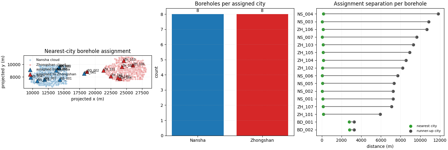
How to read this output#
A practical reading order is:
inspect the full classified CSV,
check the per-city split files,
compare the nearest distances,
look at the assignment margin.
In this lesson, most boreholes sit clearly closer to one city cloud, while the two boundary boreholes show smaller margins because both candidate cities are more competitive there.
Why this builder is useful in practice#
assign-boreholes is a support-layer command that becomes very
useful once a project starts mixing:
one external validation table,
several city-specific Stage-1 outputs,
and later city-specific evaluation workflows.
It keeps the logic simple:
load one borehole table,
resolve one or more city clouds,
compute nearest-city distances,
export one combined CSV and optional split CSVs.
That is often the cleanest way to prepare borehole validation files before later metrics or plotting commands.
Command-line usage#
The command is available through both public CLI styles:
the family-specific entrypoint,
the root
geopriordispatcher.
The exact pattern used in this lesson is:
geoprior-build assign-boreholes \
    --borehole-csv boreholes_validation.csv \
    --stage1-dir results/nansha_demo_stage1 \
    --stage1-dir results/zhongshan_demo_stage1 \
    --outdir results/borehole_assignment \
    --output-stem borehole_demo
or equivalently:
geoprior build assign-boreholes \
    --borehole-csv boreholes_validation.csv \
    --stage1-dir results/nansha_demo_stage1 \
    --stage1-dir results/zhongshan_demo_stage1 \
    --outdir results/borehole_assignment \
    --output-stem borehole_demo
You can also provide city clouds explicitly:
geoprior-build assign-boreholes \
    --borehole-csv boreholes_validation.csv \
    --city-csv nansha=results/nansha_demo_stage1/nansha_proc.csv \
    --city-csv zhongshan=results/zhongshan_demo_stage1/zhongshan_proc.csv
Or resolve them from a results layout:
geoprior-build assign-boreholes \
    --borehole-csv boreholes_validation.csv \
    --results-dir results \
    --cities nansha zhongshan
Useful optional arguments include:
--borehole-x-coland--borehole-y-colwhen the borehole table uses different coordinate names,--city-x-coland--city-y-colwhen the processed city CSV uses different coordinate names,--classified-outfor one explicit combined CSV path,--no-split-fileswhen you only want the combined output,--tie-labeland--tie-tolwhen near-equal distances should be treated as ties.
Total running time of the script: (0 minutes 0.505 seconds)