Extract a rectangular region of interest with spatial-roi

This lesson teaches how to use GeoPrior’s spatial-roi build utility.

Unlike sampling or clustering builders, this command does not try to change the statistical balance of the table. Its job is simpler and very practical: cut out one rectangular spatial window from a larger dataset.

Why this matters

Rectangular ROI extraction is useful when you want to:

• debug one local part of a large city,

• prepare a smaller teaching or benchmark subset,

• focus on one hotspot or district,

• compare the same window across several years,

• or pass only a limited area to a later workflow.

That is exactly what spatial-roi is for.

What this lesson teaches

We will:

1. build a realistic synthetic city table,

2. save it as two separate input files,

3. run the real spatial-roi builder,

4. compare the default snapped ROI with the exact-boundary ROI,

5. build one compact visual preview,

6. end with direct command-line examples.

Imports

We use the real production CLI entrypoint and the shared synthetic spatial-support helpers used elsewhere in the documentation.

from __future__ import annotations

import tempfile
from pathlib import Path

import matplotlib.pyplot as plt
from matplotlib.patches import Rectangle
import numpy as np
import pandas as pd

from geoprior.cli.build_spatial_roi import (
    build_spatial_roi_main,
)
from geoprior.scripts import utils as script_utils

Step 1 - Build one reusable synthetic city support

Instead of drawing arbitrary random coordinates, we reuse the shared spatial-support helpers. That gives us a compact city-like footprint and makes the lesson consistent with the rest of the gallery.

The parameter comments are intentionally explicit so readers can see how the synthetic spatial cloud is controlled.

Key parameters

city:

Only a label attached to the support.

center_x, center_y:

Center of the projected coordinate system.

span_x, span_y:

Half-width and half-height of the support extent.

nx, ny:

Mesh density before masking.

jitter_x, jitter_y:

Small perturbations so the support is not an exact grid.

footprint:

Shape of the retained support. zhongshan_like creates a more irregular urban footprint than a plain ellipse.

keep_frac:

Fraction of masked points to keep.

seed:

Keeps the synthetic support reproducible.

support = script_utils.make_spatial_support(
    script_utils.SpatialSupportSpec(
        city="RoiDemo",
        center_x=5_400.0,
        center_y=3_000.0,
        span_x=4_600.0,
        span_y=3_100.0,
        nx=34,
        ny=26,
        jitter_x=32.0,
        jitter_y=28.0,
        footprint="zhongshan_like",
        keep_frac=0.90,
        seed=202,
    )
)

Step 2 - Turn the support into a richer multi-year table

spatial-roi accepts an ordinary table. To make the lesson more realistic, we add:

• a time column,

• one categorical district-like field,

• and a few continuous variables.

The ROI extraction itself only uses the coordinate columns, but the important point is that all the other columns are preserved in the resulting subset.

rng = np.random.default_rng(77)

years = [2023, 2024, 2025]
frames: list[pd.DataFrame] = []

base_field = script_utils.make_spatial_field(
    support,
    amplitude=2.3,
    drift_x=0.95,
    drift_y=0.40,
    phase=0.45,
    local_weight=0.16,
)

spread_field = script_utils.make_spatial_scale(
    support,
    base=0.24,
    x_weight=0.08,
    hotspot_weight=0.06,
)

for year in years:
    step = year - years[0]
    frame = support.to_frame().copy()
    frame["year"] = int(year)

    # Simple district-like categorical partition of the city footprint.
    frame["development_zone"] = np.where(
        frame["x_norm"] > 0.62,
        "East corridor",
        np.where(frame["y_norm"] > 0.55, "North belt", "Urban core"),
    )

    # Add a few continuous columns so the extracted ROI looks like a
    # realistic analysis table rather than a coordinate-only CSV.
    frame["rainfall_mm"] = (
        1240
        + 70 * step
        + 40 * frame["y_norm"]
        + rng.normal(0.0, 12.0, len(frame))
    )
    frame["groundwater_depth_m"] = (
        8.8
        + 0.8 * frame["x_norm"]
        + 0.4 * frame["y_norm"]
        + 0.3 * step
        + rng.normal(0.0, 0.10, len(frame))
    )
    frame["subsidence_proxy_mm"] = (
        6.0
        + 1.8 * base_field
        + 2.7 * spread_field
        + 0.55 * step
        + rng.normal(0.0, 0.22, len(frame))
    )

    frames.append(frame)

full_df = pd.concat(frames, ignore_index=True)

print("Synthetic table shape:", full_df.shape)
print("")
print(full_df.head(10).to_string(index=False))

Synthetic table shape: (1086, 11)

 sample_idx   coord_x  coord_y  x_norm  y_norm    city  year development_zone  rainfall_mm  groundwater_depth_m  subsidence_proxy_mm
          0 3354.3711 867.4584  0.2805  0.1616 RoiDemo  2023       Urban core    1251.5986               9.0333               8.3842
          1 3651.1703 871.5600  0.3122  0.1623 RoiDemo  2023       Urban core    1239.6413               9.0726               8.0214
          2 3907.3201 904.3975  0.3395  0.1675 RoiDemo  2023       Urban core    1278.5531               9.1977               8.1004
          3 4160.7506 882.4783  0.3665  0.1640 RoiDemo  2023       Urban core    1227.2580               9.0794               8.4243
          4 4434.5220 883.6611  0.3958  0.1642 RoiDemo  2023       Urban core    1254.5086               9.0123               7.8218
          5 4748.0635 887.5293  0.4292  0.1648 RoiDemo  2023       Urban core    1244.8715               9.1953               7.3393
          6 4996.6863 863.9530  0.4558  0.1611 RoiDemo  2023       Urban core    1242.1890               9.1822               7.5036
          7 5208.5982 917.1658  0.4784  0.1695 RoiDemo  2023       Urban core    1259.5768               9.1977               7.6670
          8 5544.7384 860.7138  0.5143  0.1606 RoiDemo  2023       Urban core    1224.6075               9.3063               7.9484
          9 5761.8967 934.1979  0.5375  0.1722 RoiDemo  2023       Urban core    1235.0724               9.1333               7.9402

Step 3 - Save the synthetic table as two input files

The shared build-reader utilities accept one or many input files. To make that visible here, we split the city into two files and let the real command merge them again.

tmp_dir = Path(
    tempfile.mkdtemp(prefix="gp_sg_spatial_roi_")
)

west_csv = tmp_dir / "roi_demo_west.csv"
east_csv = tmp_dir / "roi_demo_east.csv"

x_mid = float(full_df["coord_x"].median())
full_df.loc[full_df["coord_x"] <= x_mid].to_csv(
    west_csv,
    index=False,
)
full_df.loc[full_df["coord_x"] > x_mid].to_csv(
    east_csv,
    index=False,
)

print("")
print("Input files")
print(" -", west_csv.name)
print(" -", east_csv.name)

Input files
 - roi_demo_west.csv
 - roi_demo_east.csv

Step 4 - Choose one requested ROI window

The command extracts a rectangular bounding box given by x_range and y_range. We intentionally choose bounds that do not align exactly with existing coordinates so the snapping behavior is visible.

Default behavior:

snap requested bounds to the nearest available coordinates.

Exact mode:

use the requested bounds exactly.

x_req = (3_020.0, 6_720.0)
y_req = (1_620.0, 4_280.0)

print("")
print("Requested ROI window")
print(f" - x_range = {x_req}")
print(f" - y_range = {y_req}")

Requested ROI window
 - x_range = (3020.0, 6720.0)
 - y_range = (1620.0, 4280.0)

Step 5 - Run the real spatial-roi builder twice

We first use the default snapped mode, then the exact mode with --no-snap-to-closest. This makes the lesson more instructive than running the builder only once.

snap_csv = tmp_dir / "roi_demo_snapped.csv"
exact_csv = tmp_dir / "roi_demo_exact.csv"

build_spatial_roi_main(
    [
        str(west_csv),
        str(east_csv),
        "--x-range",
        str(x_req[0]),
        str(x_req[1]),
        "--y-range",
        str(y_req[0]),
        str(y_req[1]),
        "--x-col",
        "coord_x",
        "--y-col",
        "coord_y",
        "--output",
        str(snap_csv),
    ]
)

build_spatial_roi_main(
    [
        str(west_csv),
        str(east_csv),
        "--x-range",
        str(x_req[0]),
        str(x_req[1]),
        "--y-range",
        str(y_req[0]),
        str(y_req[1]),
        "--x-col",
        "coord_x",
        "--y-col",
        "coord_y",
        "--no-snap-to-closest",
        "--output",
        str(exact_csv),
    ]
)

[OK] loaded 1,086 row(s) and wrote 396 ROI row(s) to /tmp/gp_sg_spatial_roi_zgkbotfa/roi_demo_snapped.csv
[OK] loaded 1,086 row(s) and wrote 396 ROI row(s) to /tmp/gp_sg_spatial_roi_zgkbotfa/roi_demo_exact.csv

Step 6 - Read the extracted tables back in

The two outputs differ only in how the bounds were interpreted.

roi_snap = pd.read_csv(snap_csv)
roi_exact = pd.read_csv(exact_csv)

print("")
print("Written files")
print(" -", snap_csv.name)
print(" -", exact_csv.name)

print("")
print("Snapped ROI")
print(roi_snap.head(8).to_string(index=False))

print("")
print("Exact ROI")
print(roi_exact.head(8).to_string(index=False))

Written files
 - roi_demo_snapped.csv
 - roi_demo_exact.csv

Snapped ROI
 sample_idx   coord_x   coord_y  x_norm  y_norm    city  year development_zone  rainfall_mm  groundwater_depth_m  subsidence_proxy_mm
         56 3678.6317 1667.5391  0.3151  0.2884 RoiDemo  2023       Urban core    1248.4245               9.2080               8.3593
         57 3827.6951 1648.9279  0.3310  0.2855 RoiDemo  2023       Urban core    1239.9210               9.1354               8.3332
         58 4101.5949 1683.6767  0.3602  0.2910 RoiDemo  2023       Urban core    1254.6335               9.1575               9.0047
         59 4655.3783 1662.2047  0.4193  0.2876 RoiDemo  2023       Urban core    1254.6778               9.2585               8.5010
         60 4942.7000 1670.4129  0.4500  0.2889 RoiDemo  2023       Urban core    1242.4392               9.2642               8.5289
         62 5502.0618 1693.2357  0.5097  0.2925 RoiDemo  2023       Urban core    1251.4842               9.3969               9.6805
         77 3020.3612 1864.4956  0.2448  0.3197 RoiDemo  2023       Urban core    1269.3408               9.2732               8.1594
         78 3321.7994 1849.7282  0.2770  0.3173 RoiDemo  2023       Urban core    1252.0279               9.0861               8.4065

Exact ROI
 sample_idx   coord_x   coord_y  x_norm  y_norm    city  year development_zone  rainfall_mm  groundwater_depth_m  subsidence_proxy_mm
         56 3678.6317 1667.5391  0.3151  0.2884 RoiDemo  2023       Urban core    1248.4245               9.2080               8.3593
         57 3827.6951 1648.9279  0.3310  0.2855 RoiDemo  2023       Urban core    1239.9210               9.1354               8.3332
         58 4101.5949 1683.6767  0.3602  0.2910 RoiDemo  2023       Urban core    1254.6335               9.1575               9.0047
         59 4655.3783 1662.2047  0.4193  0.2876 RoiDemo  2023       Urban core    1254.6778               9.2585               8.5010
         60 4942.7000 1670.4129  0.4500  0.2889 RoiDemo  2023       Urban core    1242.4392               9.2642               8.5289
         62 5502.0618 1693.2357  0.5097  0.2925 RoiDemo  2023       Urban core    1251.4842               9.3969               9.6805
         77 3020.3612 1864.4956  0.2448  0.3197 RoiDemo  2023       Urban core    1269.3408               9.2732               8.1594
         78 3321.7994 1849.7282  0.2770  0.3173 RoiDemo  2023       Urban core    1252.0279               9.0861               8.4065

Step 7 - Summarize what changed

A compact summary helps the reader see what snapping actually does.

We track:

• row counts,

• unique spatial support points,

• and the realised min/max bounds in the returned tables.

def summarize_roi(df: pd.DataFrame, label: str) -> dict[str, object]:
    return {
        "mode": label,
        "rows": int(len(df)),
        "unique_points": int(df["sample_idx"].nunique()),
        "x_min": float(df["coord_x"].min()),
        "x_max": float(df["coord_x"].max()),
        "y_min": float(df["coord_y"].min()),
        "y_max": float(df["coord_y"].max()),
        "years": ", ".join(str(y) for y in sorted(df["year"].unique())),
    }


summary = pd.DataFrame(
    [
        summarize_roi(roi_snap, "snapped"),
        summarize_roi(roi_exact, "exact"),
    ]
)

print("")
print("ROI summary")
print(summary.to_string(index=False))

ROI summary
   mode  rows  unique_points     x_min     x_max     y_min     y_max            years
snapped   396            132 3020.3612 6687.9892 1633.1354 4185.1935 2023, 2024, 2025
  exact   396            132 3020.3612 6687.9892 1633.1354 4185.1935 2023, 2024, 2025

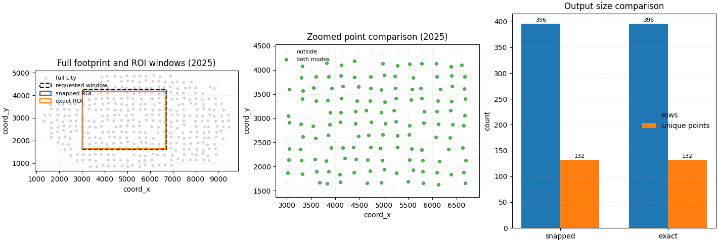
Step 8 - Build one compact visual preview

Left:

the full city footprint with the requested rectangle and the two realised ROI rectangles.

Middle:

a zoomed comparison of which points are selected by both modes, snapped-only, or exact-only.

Right:

a count comparison between the two output tables.

# Compare point membership on a single year so the map stays readable.
year_view = 2025
snap_keys = set(
    roi_snap.loc[roi_snap["year"] == year_view, "sample_idx"].tolist()
)
exact_keys = set(
    roi_exact.loc[roi_exact["year"] == year_view, "sample_idx"].tolist()
)

both_keys = snap_keys & exact_keys
snap_only = snap_keys - exact_keys
exact_only = exact_keys - snap_keys

view_df = full_df.loc[full_df["year"] == year_view].copy()
view_df["selection"] = "outside"
view_df.loc[
    view_df["sample_idx"].isin(both_keys), "selection"
] = "both"
view_df.loc[
    view_df["sample_idx"].isin(snap_only), "selection"
] = "snapped_only"
view_df.loc[
    view_df["sample_idx"].isin(exact_only), "selection"
] = "exact_only"

snap_bounds = summary.loc[summary["mode"] == "snapped"].iloc[0]
exact_bounds = summary.loc[summary["mode"] == "exact"].iloc[0]

fig, axes = plt.subplots(
    1,
    3,
    figsize=(14.2, 4.8),
    constrained_layout=True,
)

# Full support and rectangles.
ax = axes[0]
ax.scatter(
    full_df.loc[full_df["year"] == year_view, "coord_x"],
    full_df.loc[full_df["year"] == year_view, "coord_y"],
    s=9,
    alpha=0.30,
    color="0.55",
    label="full city",
)
ax.add_patch(
    Rectangle(
        (x_req[0], y_req[0]),
        x_req[1] - x_req[0],
        y_req[1] - y_req[0],
        fill=False,
        linestyle="--",
        linewidth=1.5,
        edgecolor="black",
        label="requested window",
    )
)
ax.add_patch(
    Rectangle(
        (float(snap_bounds["x_min"]), float(snap_bounds["y_min"])),
        float(snap_bounds["x_max"] - snap_bounds["x_min"]),
        float(snap_bounds["y_max"] - snap_bounds["y_min"]),
        fill=False,
        linewidth=1.7,
        edgecolor="tab:blue",
        label="snapped ROI",
    )
)
ax.add_patch(
    Rectangle(
        (float(exact_bounds["x_min"]), float(exact_bounds["y_min"])),
        float(exact_bounds["x_max"] - exact_bounds["x_min"]),
        float(exact_bounds["y_max"] - exact_bounds["y_min"]),
        fill=False,
        linewidth=1.7,
        edgecolor="tab:orange",
        label="exact ROI",
    )
)
ax.set_title(f"Full footprint and ROI windows ({year_view})")
ax.set_xlabel("coord_x")
ax.set_ylabel("coord_y")
ax.legend(frameon=False, fontsize=8)
ax.grid(True, linestyle=":", alpha=0.35)
ax.set_aspect("equal", adjustable="box")

# Zoomed selection comparison.
ax = axes[1]
colors = {
    "outside": "0.85",
    "both": "tab:green",
    "snapped_only": "tab:blue",
    "exact_only": "tab:orange",
}
labels = {
    "outside": "outside",
    "both": "both modes",
    "snapped_only": "snapped only",
    "exact_only": "exact only",
}
for key in ["outside", "both", "snapped_only", "exact_only"]:
    sub = view_df.loc[view_df["selection"] == key]
    if sub.empty:
        continue
    ax.scatter(
        sub["coord_x"],
        sub["coord_y"],
        s=18 if key != "outside" else 10,
        alpha=0.80 if key != "outside" else 0.25,
        color=colors[key],
        label=labels[key],
    )
ax.set_xlim(x_req[0] - 250.0, x_req[1] + 250.0)
ax.set_ylim(y_req[0] - 250.0, y_req[1] + 250.0)
ax.set_title(f"Zoomed point comparison ({year_view})")
ax.set_xlabel("coord_x")
ax.set_ylabel("coord_y")
ax.legend(frameon=False, fontsize=8)
ax.grid(True, linestyle=":", alpha=0.35)
ax.set_aspect("equal", adjustable="box")

# Count comparison.
ax = axes[2]
bar_x = np.arange(len(summary))
rows = summary["rows"].to_numpy(int)
pts = summary["unique_points"].to_numpy(int)
width = 0.36
ax.bar(bar_x - width / 2, rows, width=width, label="rows")
ax.bar(bar_x + width / 2, pts, width=width, label="unique points")
ax.set_xticks(bar_x)
ax.set_xticklabels(summary["mode"].tolist())
ax.set_title("Output size comparison")
ax.set_ylabel("count")
ax.legend(frameon=False)
ax.grid(True, axis="y", linestyle=":", alpha=0.35)
for i, (r, p) in enumerate(zip(rows, pts, strict=False)):
    ax.text(i - width / 2, r + 1.5, str(r), ha="center", va="bottom", fontsize=8)
    ax.text(i + width / 2, p + 1.5, str(p), ha="center", va="bottom", fontsize=8)

plt.show()

How to read this output

The main lesson is that the builder is not changing the table schema; it is only selecting a spatial window.

A useful reading order is:

1. check the requested rectangle,

2. compare the realised output bounds,

3. compare the output sizes,

4. verify that all non-spatial columns are still present.

In this example, the snapped mode uses the nearest available coordinate values, while the exact mode keeps the requested numeric limits directly. On an irregular support cloud, that can slightly change the selected rows.

Why this builder is useful in practice

spatial-roi is a strong support-layer builder when you need one local window but want to preserve the full tabular structure inside that window.

Typical uses include:

• compact local debugging datasets,

• hotspot inspection,

• district-level exports,

• or focused subsets for later plots and summaries.

Command-line usage

The same lesson can be reproduced from the terminal.

Default snapped ROI

geoprior-build spatial-roi \
    roi_demo_west.csv roi_demo_east.csv \
    --x-range 3020 6720 \
    --y-range 1620 4280 \
    --x-col coord_x \
    --y-col coord_y \
    --output roi_demo_snapped.csv

The same command through the root dispatcher

geoprior build spatial-roi \
    roi_demo_west.csv roi_demo_east.csv \
    --x-range 3020 6720 \
    --y-range 1620 4280 \
    --x-col coord_x \
    --y-col coord_y \
    --output roi_demo_snapped.csv

Exact-boundary ROI

geoprior-build spatial-roi \
    roi_demo_west.csv roi_demo_east.csv \
    --x-range 3020 6720 \
    --y-range 1620 4280 \
    --x-col coord_x \
    --y-col coord_y \
    --no-snap-to-closest \
    --output roi_demo_exact.csv

Because the shared reader accepts one or many input tables, the same command family can also be used with CSV, TSV, Parquet, Excel, JSON, Feather, or Pickle inputs.