
Note
Go to the end to download the full example code.
Build non-overlapping spatial sample batches#
This example teaches you how to use GeoPrior’s
batch-spatial-sampling build utility.
The previous spatial-sampling lesson produced one compact
sampled table. This lesson goes one step further: it produces
several non-overlapping sampled tables from the same input.
Why this matters#
Batch sampling is useful when one compact sample is not enough. Sometimes you want several small-but-representative subsets so you can:
run repeated demos or smoke tests,
compare stability across sampled subsets,
distribute work across several smaller jobs,
or prepare several compact teaching datasets without reusing the same rows every time.
That is exactly what batch-spatial-sampling is for.
Imports#
We call the real production entrypoint from the project code.
For the synthetic spatial support, we reuse the shared helpers from
geoprior.scripts.utils so the lesson remains consistent with the
rest of the documentation.
from __future__ import annotations

import tempfile
from pathlib import Path

import matplotlib.pyplot as plt
import numpy as np
import pandas as pd

from geoprior.cli.build_batch_spatial_sampling import (
    build_batch_spatial_sampling_main,
)
from geoprior.scripts.utils import (
    SpatialSupportSpec,
    make_spatial_field,
    make_spatial_scale,
    make_spatial_support,
)
Build two synthetic city supports#
We again start from SpatialSupportSpec so the user can see how a
reusable spatial support is defined.
Key parameters#
- city:
Only the city label attached to the generated support.
- center_x, center_y:
Approximate center of the synthetic projected or geographic space.
- span_x, span_y:
Half-width and half-height of the city’s extent.
- nx, ny:
Mesh density before masking.
- jitter_x, jitter_y:
Small perturbations so the support is not an exact grid.
- footprint:
Synthetic city shape. Here we use the city-like footprints.
- keep_frac:
Fraction of masked support points to keep.
- seed:
Keeps the support reproducible across doc builds.
ns_support = make_spatial_support(
    SpatialSupportSpec(
        city="Nansha",
        center_x=113.52,
        center_y=22.74,
        span_x=0.17,
        span_y=0.11,
        nx=64,
        ny=50,
        jitter_x=0.0014,
        jitter_y=0.0011,
        footprint="nansha_like",
        keep_frac=0.84,
        seed=11,
    )
)

zh_support = make_spatial_support(
    SpatialSupportSpec(
        city="Zhongshan",
        center_x=113.38,
        center_y=22.53,
        span_x=0.19,
        span_y=0.13,
        nx=66,
        ny=52,
        jitter_x=0.0015,
        jitter_y=0.0012,
        footprint="zhongshan_like",
        keep_frac=0.82,
        seed=23,
    )
)

print("Synthetic support sizes")
print(f" - Nansha   : {ns_support.sample_idx.size:,} points")
print(f" - Zhongshan: {zh_support.sample_idx.size:,} points")
Synthetic support sizes
 - Nansha   : 1,336 points
 - Zhongshan: 1,330 points
Convert the supports into a richer multi-year table#
batch-spatial-sampling operates on a regular DataFrame, so we now
build one realistic synthetic input table.
Each row will carry:
spatial coordinates,
a time stamp,
several categorical stratification fields,
one continuous response-like field,
and a unique
row_uidso we can verify that batches do not share the same sampled row.
rng = np.random.default_rng(84)

years = [2020, 2021, 2022, 2023, 2024]
frames: list[pd.DataFrame] = []

for support, amp0, drift_x, drift_y in [
    (ns_support, 6.8, 0.10, 0.08),
    (zh_support, 7.4, 0.07, 0.10),
]:
    base_mean = make_spatial_field(
        support,
        amplitude=amp0,
        drift_x=drift_x,
        drift_y=drift_y,
        phase=0.25,
        hotspot_weight=0.92,
        secondary_weight=0.56,
        ridge_weight=0.18,
        wave_weight=0.14,
        local_weight=0.06,
    )

    for year in years:
        step = year - years[0]

        scale = make_spatial_scale(
            support,
            base=0.30,
            x_weight=0.08,
            hotspot_weight=0.06,
            step_weight=0.025,
            step=step,
        )

        mean = base_mean + 0.62 * step
        noise = rng.normal(0.0, scale * 0.55)

        frame = support.to_frame().rename(
            columns={
                "coord_x": "longitude",
                "coord_y": "latitude",
            }
        )
        frame["year"] = int(year)

        # Keep a compact but meaningful set of categorical variables so
        # the lesson can show why stratification is useful.
        frame["lithology_class"] = np.where(
            frame["y_norm"] > 0.62,
            "Clay",
            np.where(frame["x_norm"] > 0.57, "Fill", "Sand"),
        )
        frame["development_zone"] = np.where(
            frame["x_norm"] + frame["y_norm"] > 1.10,
            "Urban core",
            "Expansion belt",
        )
        frame["hydro_zone"] = np.where(
            frame["y_norm"] < 0.34,
            "Low plain",
            np.where(frame["y_norm"] < 0.67, "Middle belt", "High belt"),
        )

        frame["rainfall_mm"] = (
            1260
            + 72 * step
            + 48 * frame["y_norm"]
            + rng.normal(0.0, 12.0, len(frame))
        )
        frame["subsidence_mm"] = mean + noise

        # Unique row key used only for demonstration checks after batching.
        frame["row_uid"] = [
            f"{support.city}_{idx}_{year}"
            for idx in frame["sample_idx"].to_numpy()
        ]

        frames.append(frame)

full_df = pd.concat(frames, ignore_index=True)

print("")
print("Synthetic input table")
print(full_df.head(8).to_string(index=False))
Synthetic input table
 sample_idx  longitude  latitude  x_norm  y_norm   city  year lithology_class development_zone hydro_zone  rainfall_mm  subsidence_mm       row_uid
          0   113.5074   22.6590  0.4624  0.1423 Nansha  2020            Sand   Expansion belt  Low plain    1260.3657        -0.4042 Nansha_0_2020
          1   113.4808   22.6617  0.3856  0.1542 Nansha  2020            Sand   Expansion belt  Low plain    1267.5303         0.1706 Nansha_1_2020
          2   113.4906   22.6629  0.4140  0.1595 Nansha  2020            Sand   Expansion belt  Low plain    1247.5171        -0.3128 Nansha_2_2020
          3   113.5044   22.6627  0.4537  0.1586 Nansha  2020            Sand   Expansion belt  Low plain    1271.5833         0.1742 Nansha_3_2020
          4   113.5120   22.6610  0.4760  0.1510 Nansha  2020            Sand   Expansion belt  Low plain    1246.3361        -0.3348 Nansha_4_2020
          5   113.5210   22.6606  0.5018  0.1496 Nansha  2020            Sand   Expansion belt  Low plain    1287.0786        -0.1820 Nansha_5_2020
          6   113.5295   22.6605  0.5266  0.1491 Nansha  2020            Sand   Expansion belt  Low plain    1264.6117        -0.0300 Nansha_6_2020
          7   113.5329   22.6611  0.5365  0.1517 Nansha  2020            Sand   Expansion belt  Low plain    1261.6202        -0.0895 Nansha_7_2020
Write one input file per city#
The build command uses the shared table-reader utilities, so we teach the multi-file workflow directly.
tmp_dir = Path(
    tempfile.mkdtemp(prefix="gp_sg_batch_spatial_sampling_")
)

ns_csv = tmp_dir / "nansha_spatial_panel.csv"
zh_csv = tmp_dir / "zhongshan_spatial_panel.csv"

full_df.loc[full_df["city"] == "Nansha"].to_csv(
    ns_csv,
    index=False,
)
full_df.loc[full_df["city"] == "Zhongshan"].to_csv(
    zh_csv,
    index=False,
)

print("")
print("Input files")
print(" -", ns_csv.name)
print(" -", zh_csv.name)
Input files
 - nansha_spatial_panel.csv
 - zhongshan_spatial_panel.csv
Run the real batch-spatial-sampling builder#
We ask the command to:
read both city tables,
produce four non-overlapping sampled batches,
preserve balance across city, year, and lithology class,
write one stacked output table,
and also write one file per batch into a split directory.
Here sample-size is the total sampling size across all
batches, not the size of each batch individually.
stacked_csv = tmp_dir / "batch_spatial_sampling_gallery.csv"
split_dir = tmp_dir / "batch_files"

build_batch_spatial_sampling_main(
    [
        str(ns_csv),
        str(zh_csv),
        "--sample-size",
        "0.24",
        "--n-batches",
        "4",
        "--stratify-by",
        "city",
        "year",
        "lithology_class",
        "--spatial-cols",
        "longitude",
        "latitude",
        "--spatial-bins",
        "8",
        "7",
        "--method",
        "relative",
        "--min-relative-ratio",
        "0.03",
        "--random-state",
        "42",
        "--batch-col",
        "batch_id",
        "--output",
        str(stacked_csv),
        "--split-dir",
        str(split_dir),
        "--split-prefix",
        "spatial_batch_",
        "--verbose",
        "1",
    ]
)
Generating stratification keys for 13,330 records...
 This may take some time. Please be patient...
Stratification keys generated successfully for 13,330 records.

Creating 4 stratified batches with a total of 3,199 samples...

Batch Sampling Progress:   0%|                            | 0/4 [00:00<?, ?it/s]
Batch Sampling Progress:  25%|#####               | 1/4 [00:00<00:00,  5.66it/s]
Batch Sampling Progress:  50%|##########          | 2/4 [00:00<00:00,  5.64it/s]
Batch Sampling Progress:  75%|###############     | 3/4 [00:00<00:00,  5.65it/s]
Batch Sampling Progress: 100%|####################| 4/4 [00:00<00:00,  5.59it/s]
Batch Sampling Progress: 100%|####################| 4/4 [00:00<00:00,  5.61it/s]

Batch sampling completed. 4 batches created.
[OK] loaded 13,330 row(s), created 4 batch(es), and wrote 3,230 sampled row(s) to /tmp/gp_sg_batch_spatial_sampling_5w2kjtvm/batch_spatial_sampling_gallery.csv
[OK] also wrote 4 per-batch file(s) to /tmp/gp_sg_batch_spatial_sampling_5w2kjtvm/batch_files
Inspect the written outputs#
The command writes:
one stacked table containing every sampled row,
and, when
--split-diris used, one file per batch.
stacked_df = pd.read_csv(stacked_csv)
batch_files = sorted(split_dir.glob("spatial_batch_*.csv"))
batch_tables = [pd.read_csv(p) for p in batch_files]

print("")
print("Written files")
print(" -", stacked_csv.name)
for p in batch_files:
    print(" -", p.relative_to(tmp_dir))

print("")
print("Stacked batch table")
print(stacked_df.head(10).to_string(index=False))
Written files
 - batch_spatial_sampling_gallery.csv
 - batch_files/spatial_batch_001.csv
 - batch_files/spatial_batch_002.csv
 - batch_files/spatial_batch_003.csv
 - batch_files/spatial_batch_004.csv

Stacked batch table
 batch_id  sample_idx  longitude  latitude  x_norm  y_norm   city  year lithology_class development_zone  hydro_zone  rainfall_mm  subsidence_mm          row_uid
        1        1059   113.4420   22.7783  0.2730  0.6710 Nansha  2020            Clay   Expansion belt   High belt    1293.3040         2.0112 Nansha_1059_2020
        1        1096   113.4422   22.7806  0.2736  0.6812 Nansha  2020            Clay   Expansion belt   High belt    1281.1165         2.2193 Nansha_1096_2020
        1        1233   113.4752   22.7994  0.3693  0.7645 Nansha  2020            Clay       Urban core   High belt    1299.6382         2.2006 Nansha_1233_2020
        1        1065   113.4790   22.7760  0.3804  0.6608 Nansha  2020            Clay   Expansion belt Middle belt    1275.5686         3.6701 Nansha_1065_2020
        1         990   113.4722   22.7690  0.3605  0.6301 Nansha  2020            Clay   Expansion belt Middle belt    1297.8654         3.7624  Nansha_990_2020
        1        1205   113.5161   22.7954  0.4878  0.7469 Nansha  2020            Clay       Urban core   High belt    1290.7332         2.0745 Nansha_1205_2020
        1        1172   113.5117   22.7905  0.4750  0.7251 Nansha  2020            Clay       Urban core   High belt    1293.4455         2.6689 Nansha_1172_2020
        1        1170   113.5004   22.7931  0.4423  0.7365 Nansha  2020            Clay       Urban core   High belt    1298.8818         2.8452 Nansha_1170_2020
        1        1312   113.5122   22.8098  0.4765  0.8107 Nansha  2020            Clay       Urban core   High belt    1295.5397         1.5163 Nansha_1312_2020
        1        1113   113.5655   22.7807  0.6310  0.6819 Nansha  2020            Clay       Urban core   High belt    1281.1163         2.6213 Nansha_1113_2020
Prove that batches are distinct and still representative#
A useful lesson should not stop after a successful write. We also inspect whether the output actually delivers what the command promises.
We check three things:
batch sizes,
distribution by city and year,
overlap between batches using
row_uid.
batch_sizes = (
    stacked_df.groupby("batch_id").size().rename("n_rows").reset_index()
)

batch_city = (
    stacked_df.groupby(["batch_id", "city"])
    .size()
    .rename("n_rows")
    .reset_index()
)

batch_year = (
    stacked_df.groupby(["batch_id", "year"])
    .size()
    .rename("n_rows")
    .reset_index()
)

# Pairwise overlap matrix based on the unique row id.
row_sets = {
    int(i + 1): set(tab["row_uid"])
    for i, tab in enumerate(batch_tables)
}

batch_ids = sorted(row_sets)
overlap = np.zeros((len(batch_ids), len(batch_ids)), dtype=int)

for i, bi in enumerate(batch_ids):
    for j, bj in enumerate(batch_ids):
        overlap[i, j] = len(row_sets[bi] & row_sets[bj])

overlap_df = pd.DataFrame(
    overlap,
    index=[f"Batch {i}" for i in batch_ids],
    columns=[f"Batch {i}" for i in batch_ids],
)

all_unique = stacked_df["row_uid"].nunique()
all_rows = len(stacked_df)

print("")
print("Batch sizes")
print(batch_sizes.to_string(index=False))

print("")
print("Rows by batch and city")
print(batch_city.to_string(index=False))

print("")
print("Rows by batch and year")
print(batch_year.to_string(index=False))

print("")
print("Pairwise overlap matrix based on row_uid")
print(overlap_df.to_string())

print("")
print(
    "Uniqueness check: "
    f"{all_unique:,} unique sampled rows out of {all_rows:,} stacked rows"
)
Batch sizes
 batch_id  n_rows
        1     820
        2     795
        3     820
        4     795

Rows by batch and city
 batch_id      city  n_rows
        1    Nansha     400
        1 Zhongshan     420
        2    Nansha     390
        2 Zhongshan     405
        3    Nansha     400
        3 Zhongshan     420
        4    Nansha     400
        4 Zhongshan     395

Rows by batch and year
 batch_id  year  n_rows
        1  2020     164
        1  2021     164
        1  2022     164
        1  2023     164
        1  2024     164
        2  2020     159
        2  2021     159
        2  2022     159
        2  2023     159
        2  2024     159
        3  2020     164
        3  2021     164
        3  2022     164
        3  2023     164
        3  2024     164
        4  2020     159
        4  2021     159
        4  2022     159
        4  2023     159
        4  2024     159

Pairwise overlap matrix based on row_uid
         Batch 1  Batch 2  Batch 3  Batch 4
Batch 1      820        0        0        0
Batch 2        0      795        0        0
Batch 3        0        0      820        0
Batch 4        0        0        0      795

Uniqueness check: 3,230 unique sampled rows out of 3,230 stacked rows
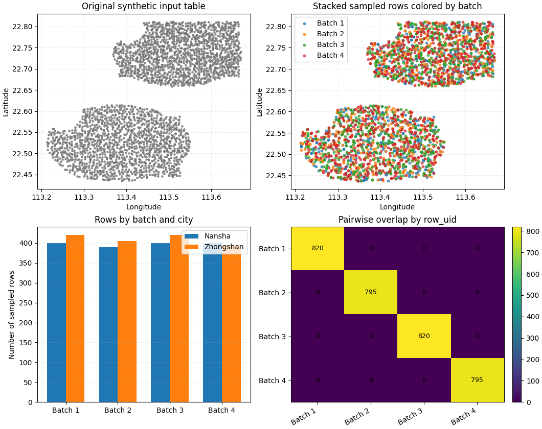
Build one compact visual preview#
- Top-left:
the full spatial footprint in light gray.
- Top-right:
the stacked sampled output colored by batch.
- Bottom-left:
counts by batch and city.
- Bottom-right:
pairwise overlap heatmap. Off-diagonal zeros are what we want.
fig, axes = plt.subplots(
    2,
    2,
    figsize=(10.6, 8.4),
    constrained_layout=True,
)

batch_colors = {
    1: "tab:blue",
    2: "tab:orange",
    3: "tab:green",
    4: "tab:red",
}

# Full input footprint.
ax = axes[0, 0]
ax.scatter(
    full_df["longitude"],
    full_df["latitude"],
    s=5,
    alpha=0.22,
    color="0.45",
)
ax.set_title("Original synthetic input table")
ax.set_xlabel("Longitude")
ax.set_ylabel("Latitude")
ax.grid(True, linestyle=":", alpha=0.4)

# Stacked batches.
ax = axes[0, 1]
for batch_id in sorted(stacked_df["batch_id"].unique()):
    sub = stacked_df.loc[stacked_df["batch_id"] == batch_id]
    ax.scatter(
        sub["longitude"],
        sub["latitude"],
        s=10,
        alpha=0.70,
        label=f"Batch {int(batch_id)}",
        color=batch_colors[int(batch_id)],
    )
ax.set_title("Stacked sampled rows colored by batch")
ax.set_xlabel("Longitude")
ax.set_ylabel("Latitude")
ax.legend(loc="best")
ax.grid(True, linestyle=":", alpha=0.4)

# Counts by batch and city.
ax = axes[1, 0]
wide_city = batch_city.pivot(
    index="batch_id",
    columns="city",
    values="n_rows",
).fillna(0)
xx = np.arange(len(wide_city.index))
bar_w = 0.36
cities = list(wide_city.columns)
for k, city in enumerate(cities):
    ax.bar(
        xx + (k - 0.5) * bar_w,
        wide_city[city].to_numpy(),
        width=bar_w,
        label=city,
    )
ax.set_title("Rows by batch and city")
ax.set_ylabel("Number of sampled rows")
ax.set_xticks(xx)
ax.set_xticklabels([f"Batch {int(i)}" for i in wide_city.index])
ax.legend(loc="best")
ax.grid(True, axis="y", linestyle=":", alpha=0.4)

# Pairwise overlap heatmap.
ax = axes[1, 1]
im = ax.imshow(overlap_df.to_numpy(), aspect="auto")
ax.set_title("Pairwise overlap by row_uid")
ax.set_xticks(np.arange(len(overlap_df.columns)))
ax.set_yticks(np.arange(len(overlap_df.index)))
ax.set_xticklabels(overlap_df.columns, rotation=30, ha="right")
ax.set_yticklabels(overlap_df.index)
for i in range(overlap_df.shape[0]):
    for j in range(overlap_df.shape[1]):
        ax.text(
            j,
            i,
            int(overlap_df.iloc[i, j]),
            ha="center",
            va="center",
            fontsize=9,
        )
fig.colorbar(im, ax=ax, fraction=0.048, pad=0.04)
<matplotlib.colorbar.Colorbar object at 0x749e5682ede0>
How to read this output#
The point of batch sampling is not just to create many files. The important thing is that the batches remain useful.
In this preview, the desirable pattern is:
each batch still covers both cities,
each batch still contains multiple years,
the stacked table remains representative of the original footprint,
and the off-diagonal overlap cells stay at zero.
That combination makes batch-spatial-sampling a practical builder
for repeated experiments, debugging, teaching, and lightweight batch
workflows.
Command-line usage#
The same workflow can be run directly from the command line.
Family entry point:
geoprior-build batch-spatial-sampling \
    nansha_spatial_panel.csv \
    zhongshan_spatial_panel.csv \
    --sample-size 0.24 \
    --n-batches 4 \
    --stratify-by city year lithology_class \
    --spatial-cols longitude latitude \
    --spatial-bins 8 7 \
    --method relative \
    --min-relative-ratio 0.03 \
    --random-state 42 \
    --batch-col batch_id \
    --output batch_spatial_sampling_gallery.csv \
    --split-dir batch_files \
    --split-prefix spatial_batch_
Root entry point:
geoprior build batch-spatial-sampling \
    nansha_spatial_panel.csv \
    zhongshan_spatial_panel.csv \
    --sample-size 0.24 \
    --n-batches 4 \
    --stratify-by city year lithology_class \
    --spatial-cols longitude latitude \
    --spatial-bins 8 7 \
    --method relative \
    --min-relative-ratio 0.03 \
    --random-state 42 \
    --batch-col batch_id \
    --output batch_spatial_sampling_gallery.csv \
    --split-dir batch_files \
    --split-prefix spatial_batch_
The shared data-reader arguments still apply here, so the command can
also read one or many input tables in CSV / TSV / Parquet / Excel /
JSON / Feather / Pickle form, and Excel paths may use selectors such
as input.xlsx::Sheet1.
Total running time of the script: (0 minutes 2.291 seconds)